
In the rest of this chapter, we’ll discuss the tools that you can use to adjust the colors in an image. Here we delve into the Color chooser, Levels, and Curves tools.
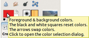
The Color chooser is the main tool for choosing a color for any painting tool. To open the Color chooser from the Toolbox, click one of the rectangles that display the current foreground and background colors, as shown in (Figure 12-42).
The Color chooser appears as shown in Figure 12-43. This dialog is packed with features, so we’ll break our discussion into several areas and look at them separately.
The top-right quadrant of the dialog contains six sliders corresponding to the channels in the HSV and RGB models. To the right of the sliders are counters that you can use to make precise changes. The radio buttons on the left are related to the first tab in the top-left quadrant, the one with Wilber’s head displayed on it. If any of the other tabs are selected, these buttons are not active.
The sliders are correlated, so if we move one of them, several others are also affected. For example, moving the S slider also changes all the RGB sliders. Moving one of the RGB sliders changes the H slider and can also change the S and V sliders, depending on their initial values. The color spectrum for the sliders changes to display the effect based on the current selection. Only the H slider always displays the same rainbow of colors.
The bottom-right quadrant of the dialog contains a number of controls. The HTML NOTATION field contains the hexadecimal representation of the current color in HTML code. This code is composed of three groups of two hexadecimal digits, representing the values of the three RGB channels. If we choose a color elsewhere in the dialog, the code will change to match, but we can also type a number into the field and look at the result, or we can even type in a color name. If we type the beginning of a name, all the available names that begin with those letters are displayed, as shown in Figure 12-44.
The small button to the right of the field is used to select a color from an image or from anywhere on the screen. If we click this button, the mouse pointer icon becomes an eyedropper. When we click somewhere on the screen (even outside of a GIMP window), the corresponding pixel color is selected for the Color chooser, and this color defines the value of the six sliders and the HTML notation field.
Below this field are 12 colored buttons that represent the color history. The button on the left with a > sign is used to add the current color to this history and remove the oldest color (the bottom-right one). If we click any of these buttons, its color becomes the current one.
The three buttons in the bottom-right corner of the dialog are mostly self-explanatory. RESET changes the current color to black but does not affect the history.
The bottom-left quadrant of the dialog contains only three controls. CURRENT and OLD represent, respectively, the current color as defined in the Color chooser dialog and the color defined before that. Click and drag the color from either of these two buttons to an image to fill the current selection. The HELP button does what you’d expect.
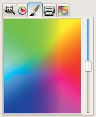
The top-left quadrant contains a rectangular display and five tabs, which give five different ways to finely tune the desired color. Figure 12-43 shows the Wilber tab, the only one that uses the six radio buttons to the left of the HSV and RGB sliders. Here, the selected radio button is H, which means the spectrum to the right of the large rectangular area shows the Hue scale. The pointer in this display indicates the current hue, whereas the rectangle on the left represents the possible variations of saturation and value when this hue is chosen. If we click this rectangle, we choose a specific value (in the horizontal scale) and a specific saturation (in the vertical scale). Two perpendicular lines cross at the chosen point, and the sliders on the right side of the dialog change to reflect the new saturation and value.


Selecting a different radio button changes the rectangular display on the left. For example, Figure 12-45 shows the display when the B (blue) radio button has been selected. The thin vertical rectangle allows us to choose the quantity of blue, and the large rectangle allows us to adjust the quantities of red and green. Occasionally, the combination that’s activated when you check the B radio button is more convenient, but usually the default (H) works best.
The Triangle tab has an icon showing a thumbnail of that tab’s display (Figure 12-46). This tab offers another graphical way to choose the color using the HSV model. Clicking the hue circle selects the H component. A click in the triangle then changes the values of the S and V components. At one of the triangle’s points, S is 0; at another point, V is 0; at the final point, both are at the maximum (100). Some people find this tab more intuitive than the Wilber tab.

The tab with a paintbrush icon behaves like a simulation of watercolor painting (Figure 12-47). A click anywhere in the rectangle adds a small quantity of that color to the current one. The vertical slider sets the quantity of color being added, from 0 at the bottom to the maximum at the top. Because colors are added to the existing color, this tab uses the CMY model, and the color obtained becomes stronger the more we click. If we click one of the rectangle’s sides, the saturation increases. If we click in the center of the rectangle, the value decreases. This tab is especially useful for building a light color, like a pastel, beginning with a full white.

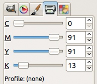
The tab marked with a printer icon contains options based on the CMYK color model (Figure 12-48). This tab is useful mainly for gathering information about how the colors will be mixed when printing rather than as a way to adjust a color, particularly because you can’t automatically change the CMY channels when changing the K channel, which is a common printing adjustment.
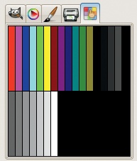
The remaining tab has an icon showing a finger on a palette (Figure 12-49). The center square shows the contents of the current palette, a concept explained in 22.7 Building New Palettes. The only colors you can choose are from this palette, but you can change the palette in the Palettes dialog, which you open via Image: Windows > Dockable Dialogs > Palettes.
Access a simplified dockable dialog for choosing colors by selecting Image: Windows > Dockable dialogs > Colors, as shown in Figure 12-50. The Colors dialog is a modified version of the left portion of the Color chooser. The Wilber tab contains six buttons on the right, used to choose the color model and the master channel. The Triangle, Watercolor, Printer, and Palette tabs are identical to those on the Color chooser. The last tab is a slightly modified version of the right portion of the Color chooser dialog (Figure 12-51).


The bottom of the Colors dialog contains several useful buttons. On the left are the buttons for setting the foreground and background colors. On the right is the button for applying the eyedropper and the field containing the HTML notation for the current color.
The Levels tool, opened by selecting Image: Colors > Levels or Image: Tools > Color Tools > Levels, is one of the most useful tools in GIMP for photo processing. In a nutshell, use the Levels tool (and the Curves tool, discussed in the next section) to adjust the relationship between initial pixel values (the input) and pixel values in the new, transformed image (the output). The Levels tool dialog is shown in Figure 12-52.

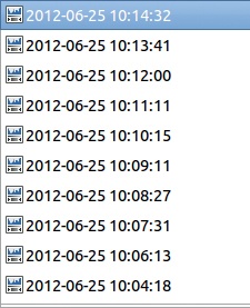
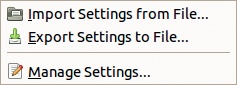
The PRESETS field at the top of the Levels dialog opens a menu of previously saved settings. The settings are identified in ISO format by the date and time they were saved (see Figure 12-53). The plus sign on the right saves the current settings. This is more convenient than remembering the ISO date and time when you used a specific setting. Named settings are listed at the end of the saved settings. The same capabilities are available in the other color tools. The small triangle on the far right opens the menu shown in Figure 12-54. Use the first two entries to import or export settings to or from a file. The last entry opens the dialog shown in Figure 12-55, which lists the saved settings and contains three buttons to import settings, export settings, and delete the selected settings.

The next line of the Levels dialog contains a menu to select the Channel that will be affected. The choices are Value, Red, Green, Blue, and Alpha (if an Alpha channel is available). When you select the Value channel, all three color channels change. The Value channel is the only channel available for a grayscale image. The RESET CHANNEL button resets the selected channel to its initial value without affecting any changes made elsewhere in the dialog.
The two buttons on the right set the characteristic of the histogram shown below. The histogram is a way to display the frequency of different values in the chosen channel. In 8-bit depth representation, there are 256 different values, from 0 on the left to 255 on the right. The height of a bar in the graph is proportional to the number of pixels in the image with this value. If the leftmost button is pressed, the peak corresponds literally to the number of pixels, whereas in the logarithmic histogram, which you select with the rightmost button, the values are calculated using a logarithm. As Figure 12-56 shows, the logarithmic histogram better illustrates variations in the low values, whereas the linear histogram (shown in Figure 12-52) exaggerates the peaks.
The purpose of the Levels tool is to change the histogram by assigning new values to certain pixels. Generally, images look best when pixels are distributed across the full range. As you can see, the values greater than 200 are not represented at all in the example we’ve used.
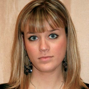
Just under the histogram are three movable triangles. The black one on the left corresponds to the black point: All pixels with a value less than or equal to the position of this triangle are set to 0 (i.e., black for color channels or full transparency for the Alpha channel). When this point moves to the right, more pixels become black, which is generally only beneficial if the histogram is empty on the left. The white triangle on the right corresponds to the white point: All pixels with a value greater than or equal to the position of that triangle are set to 255 (i.e., the maximum). Our example image would benefit from this adjustment because values greater than 200 are not represented at all. If we move the white triangle to 200, the full range of available values is represented in the image, which improves the contrast. The result is shown in Figure 12-57, which you can compare to the original image, shown in Figure 12-8.
The middle, gray triangle corresponds to the midpoint. Moving it to the left makes the image lighter in the Value channel, more saturated in a color channel, or more opaque in the Alpha channel. Moving it to the right has the opposite effect. This slider changes the value of the Gamma factor, or Gamma correction, which specifies the shape of the answering curve. The answering curve represents the relationship between the input (initial pixel) and the output (new pixel) values. If Gamma = 1, the curve is a straight line. Increasing Gamma makes the curve convex, and decreasing it makes the curve concave.
Instead of moving one of the triangles by hand, we can also change the corresponding numeric field. Additionally, two eyedroppers, one for the black point and the other for the white point, are available. By clicking one of them and then clicking in the image on a pixel of the corresponding shade, we can adjust the triangles so they bracket the values that are represented in the image.
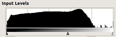
All the settings covered so far deal with the INPUT LEVELS, which enlarge the range of pixel values in the image to build a new image. Just below those controls are two triangles that alter the OUTPUT LEVELS. Moving the OUTPUT LEVELS triangles toward each other restricts the range of possible values. In the Value channel, for example, this reduces the image contrast, making the image duller, as shown in Figure 12-58.
![after restricting the output levels to [100 to 200]](http://imgdetail.ebookreading.net/design/7/9781457172410/9781457172410__the-book-of__9781457172410__httpatomoreillycomsourcenostarchimages1455570.png.jpg)

If we move the white triangle to the left side and the black triangle to the right side, then we invert the image, as illustrated in Figure 12-59. Doing this accomplishes the same thing as applying Image: Colors > Invert, except that when using the Levels tool, we can invert each of the RGB color channels separately.
So far we’ve discussed the manual settings, which alter only the selected channel. The Levels tool also includes some automatic settings, which act on all channels at the same time. The simplest and most useful of these is the AUTO button, which extends the input range of the three color channels as far as possible. Figure 12-60 shows the result for our image. Generally this improves the image, but in this example, the change is too dramatic.


The three eyedroppers on the right, like the histogram eyedroppers, can be used to select the black and white points and also a midpoint in the image. But unlike the histogram eyedroppers, these eyedroppers change all the channels, which can lead to strange and unnatural effects. Note that the order in which these points are picked is significant, and picking them all is not necessary. Generally, the midpoint is the most difficult to pick accurately.
Although the Levels tool is, by default, not accessed from the Toolbox (change this in the Image: Edit > Preferences dialog, TOOLBOX entry), it does have Toolbox options, which appear when the tool is selected. These are shown in Figure 12-61. The HISTOGRAM SCALE radio buttons do the same thing as the buttons at the top right of the Levels dialog. The SAMPLE AVERAGE option, if checked, sets the radius of the area used to pick a color in the image when using one of the eyedroppers. This square appears if you press the mouse button when clicking the image with the eyedropper selected.
Use the Curves tool to make the same adjustments as the Levels tool, but the Curves tool offers more control. Below the three eyedroppers in the Levels dialog is an EDIT THESE SETTINGS AS CURVES button, which retains any changes that were made in the Levels dialog and applies the Curves tool. The PREVIEW button allows you to see the effect of your changes and should always be checked. The four buttons at the bottom of the Levels dialog are self-explanatory.
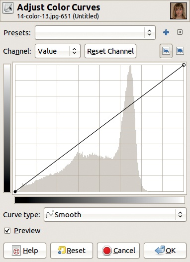
The Curves tool is found via Image: Colors > Curves or Image: Tools > Color Tools > Curves and opens the dialog shown in Figure 12-62. The Curves tool’s effect is similar to that of the Levels tool, but it offers fewer automatized options and more control.
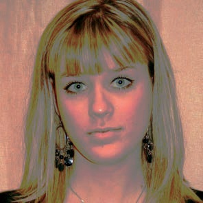
The top and the bottom of the Curves dialog are the same as the Levels dialog. In the rectangle at the center of the Curves dialog, you’ll see an image of the histogram. The diagonal of this rectangle represents the answering curve. Input values vary horizontally, and output values vary vertically. Initially, the input and output values are equal. When the mouse pointer is in the rectangle, its coordinates are displayed in the top-left corner.


By clicking and dragging the answering curve, we can change its shape. If the CURVE TYPE button shows SMOOTH, as it does by default, the curve, which remains smooth, is adjusted to pass by the points added, as shown in Figure 12-63. These points, called anchors, are automatically added every time you click in the histogram. The current anchor is a black dot. Move it by clicking and dragging or by using the up and down arrow keys on the keyboard. Press ![]() to move the arrow keys by 15 pixels at a time, rather than the default of 1 pixel. The left and right arrow keys select the next anchor in the corresponding direction. If you click near an existing anchor, you can drag it to another position, thus changing the curve. To remove an anchor, drag it into one of the other anchors.
to move the arrow keys by 15 pixels at a time, rather than the default of 1 pixel. The left and right arrow keys select the next anchor in the corresponding direction. If you click near an existing anchor, you can drag it to another position, thus changing the curve. To remove an anchor, drag it into one of the other anchors.
While the tool is in use, the mouse pointer takes the form of an eyedropper when you hover over the image. If you click the image, a vertical line appears in the Curves dialog at the value of the clicked pixel. ![]() -clicking creates an anchor in the selected channel, and
-clicking creates an anchor in the selected channel, and ![]() -clicking creates an anchor in all the channels. The anchor is inserted only when the mouse button is released, so we can drag the point around the image to find a target value.
-clicking creates an anchor in all the channels. The anchor is inserted only when the mouse button is released, so we can drag the point around the image to find a target value.
If the CURVE TYPE is set to FREEHAND, the curve is built by clicking and dragging in the rectangle and generally comes out jagged, as shown in Figure 12-64. The result is also more difficult to control, as illustrated in Figure 12-65. But if we then choose SMOOTH as the curve type, the curve is automatically smoothed, and the necessary anchors are added.
The options for the Curves tool are the same as for the Levels tool (see Figure 12-61).
The Curves tool does not have any automatic controls and can be more difficult to master than the Levels tool, but it allows for more precise color handling. If we keep the curve straight and move only its end anchors horizontally, the effect is the same as moving the end triangles under INPUT LEVELS in the Levels tool. Moving them vertically has the same effect as moving the triangles under OUTPUT LEVELS. Adding an anchor in the middle of the curve and moving it vertically does the same thing as moving the middle triangle in the Levels tool and is a more intuitive visualization of the Gamma value.
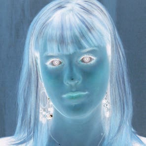
Inverting the curve by putting the left (lower) anchor in the top-left corner and the right (upper) anchor in the bottom-right corner results in a negative image, as shown in Figure 12-66. We can also do this in one channel only, with strange and colorful results. If we change the curves of individual color channels, they appear in their respective colors on the histogram, whereas the current curve is always black. These colored curves are not displayed when the Value channel is selected. Adjusting the shape of the curve can be tricky. Deforming the curve too much is easy and results in exaggerated, unnatural colors.