
Scanning is the conversion of an image to a digital representation using a specific device called a scanner. The process is also called digitizing or digitization.
An image scanner is an independent device that connects to the computer by a USB or an IEEE 1394 (Firewire) connection. In this book, we cover only the flatbed type, where the document is placed on glass and the charged coupled device (CCD) sensors move across the glass while the document is lit. The same manufacturers that make printers (such as Canon and Epson) generally also make scanners. The prices are in the same range, and multifunction devices in which a scanner and printer are combined are more and more common, including in low-cost models.
Most people buy a scanner to digitize photographs or sketches, so, for most people, an automatic feeder is unnecessary and a letter-size (or A4) glass size is sufficient. If you need to scan a large quantity of documents, you may consider buying a scanner with an automatic feeder, and if you’re an artist who works in large format, you may need a larger glass size. Many people want to scan photographic negatives or slides, which requires a specific device lit from behind; look for this capability in the scanner’s specifications.
Scanning speed is generally not very important, as long as scanning a normal-sized photograph does not take more than a minute. Scanning resolution is more important, but be warned that, as always with numeric information, resolution is used as a marketing point— a larger number is not necessarily better. A scanner has an intrinsic maximum resolution, depending on the number of CCD cells that compose the sensor array. Larger resolutions can be obtained by interpolation, which means they are a digital simulation of a higher resolution, which can also be done in GIMP. The physical, true resolution of a scanner is called the optical resolution, and only the optical resolution should be considered when comparing different models.
Actually, a large resolution is often not needed. If you intend to print the scanned image in the same size, 300 ppi (pixels per inch) is enough. If you intend to enlarge the image a lot—for example, the original is a 35 mm slide and you want to print it in letter-size format— 1200 ppi is probably enough. So resolutions of 4800 or 9600 ppi, frequently advertised for scanners, are not only artificially inflated but also useless for most people.
The most important factors to take into account when buying a scanner are its precision and fidelity in rendering the values and colors of the image’s pixels. Look at websites that compare the capabilities, performance, and prices of various scanner models.
If you are a GNU/Linux user, we recommend looking at the Scanner Access Now Easy, or SANE, website (http://www.sane-project.org/) to make sure a scanner model will be recognized on your platform. Don’t worry if you cannot buy the most recent scanner with all the bells and whistles: The bells and whistles are often useless, and the standard model, when correctly handled by SANE, will meet all your needs.
What exactly is SANE all about? All too frequently, scanner manufacturers build their devices without any thought to free and open source software. They provide drivers and applications only for Windows and Mac operating systems. The goal of the SANE project is to provide a free software version of the drivers for as many scanner models as possible. It constitutes a front-end for the scanner, which also requires a back-end to handle the digitized image. Several back-ends are available for GNU/Linux and Mac OS but not for Windows. Windows users can use the application shipped with the scanner, or they can use a client back-end, which gets its information from a GNU/Linux server running SANE, or from a SANE to TWAIN converter application.
Scanners are generally sold with accompanying software on CDs. Some come with trial or feature-limited versions of commercial image-processing applications, but since we’re using GIMP, we don’t need them. The scanner comes with its own specific application as well, which allows you to use its unique front panel buttons. You can use the scanner without these buttons without any real problem; they’re designed to make the scanner faster or easier to use but are not the only way to interface with it. For the purposes of this book, we want to digitize a picture so it’s as unchanged as possible, and then we want to process it in GIMP.
If GIMP is installed without any additional plug-ins, it can’t communicate with a scanner. Several scanner plug-ins are available for GIMP, but XSane is the best-developed and maintained tool. The XSane package is available for most GNU/Linux distributions, and installing it also installs the XSane plug-in for GIMP. We’ll be using the XSane plug-in for scanning in this chapter. If you’re using different software, the interface will be different, but similar options should be available.
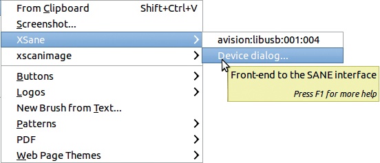
Once you’ve installed the plug-in and restarted GIMP, you’ll find XSane in the Image: File > Create menu, as shown in Figure 19-3. The first entry is the only one most users will need, but if you have two scanners, or a scanner and a webcam, you’ll see additional entries that let you choose which device will be the image source. A temporary window appears first, telling the tool is scanning for devices. If no scanner is available, an error window appears. Note that XSane can also use a webcam as input, but we’ll not consider this capability.
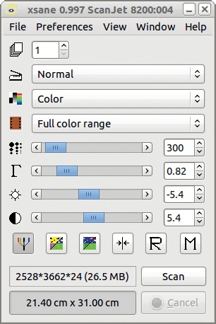
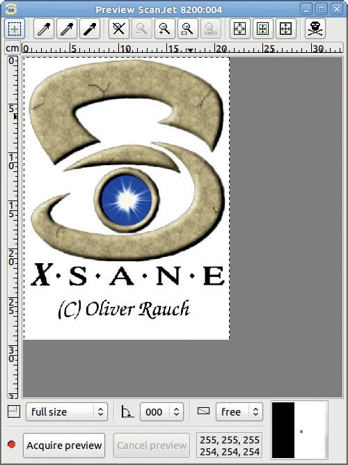
When you select XSane from the Image: File > Create menu, you’ll normally see two different dialogs. Figure 19-4 shows the main dialog, which has most of the controls and parameters. For that reason, we call it the Control window. Figure 19-5 shows the preview window, which is especially useful for selecting a subsection of the image to scan.
Other SANE back-ends have similar dialogs and controls.
First, place a photograph or drawing on the scanner glass. If the picture is on thin paper, place a black sheet on top of it, especially if there is anything on the reverse side of the paper.
Adjust the controls in the XSane control window if you’d like to and then acquire a preview by clicking the corresponding button in the preview window.
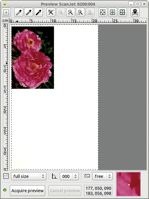
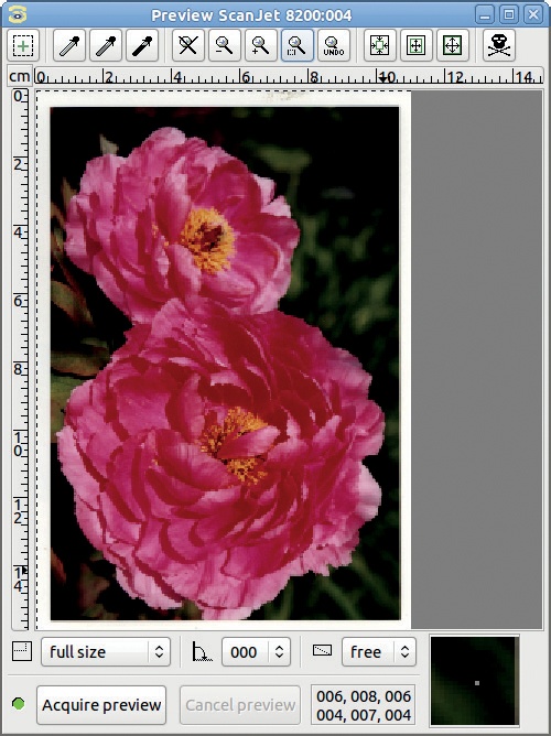
Figure 19-6 shows our initial image preview. The preview window is square to accommodate any orientation that you choose for the scan. Change the orientation using the middle button in the second row of buttons from the bottom. The large dashed rectangle is what the scanner thinks the image size is. Fortunately, we can change it by clicking and dragging the sides or corners of this rectangle. It is best to delimit a rectangle that’s slightly larger than the image because the scanner doesn’t always capture precisely what’s in the rectangle. Figure 19-7 shows a much better preview. To get this preview, we dragged the rectangle so it outlined the photograph and then clicked ZOOM INTO THE SELECTED AREA (the button with a magnifying glass and a plus sign).
Let’s take a look at the other buttons at the top of the preview window. The button with the plus sign at the far left is used for batch processing. The three eyedropper buttons are used to adjust the levels, as in GIMP. The next five buttons control the zoom. From left to right, they are: use the full scan area (no zoom), zoom 20% out, click at the position to zoom to, zoom into the selected area, and undo the last zoom. The three rectangular buttons that follow are, from left to right, autoselect the scan area, autoraise the scan area, and select the visible area. The intriguing button on the far right, the one that looks like a skull and crossbones, deletes everything that’s stored in the preview cache. Press it each time you start a new scan to be sure that all the previews of images that you scanned in the past have been cleared.
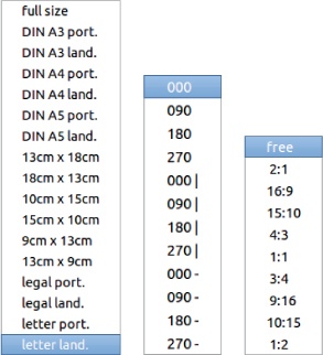
Below the preview are two rows of buttons. The upper-row buttons control the area to be scanned. Each opens a menu:
The preset areas are shown in Figure 19-8 (left). These presets allow you to select some standard dimensions automatically.
The rotation angles are shown in Figure 19-8 (center). They are all multiples of 90° with three variants. The minus signs indicate the image will be mirrored horizontally, and the pipes indicate it will be mirrored vertically.
The aspect ratios are shown in Figure 19-8 (right). Use the aspect ratios to set the relationship of width to height and thus control the shape of the region you select to scan.
Although you can use XSane to adjust the image, we recommend scanning the image as is and then making any necessary adjustments in GIMP.
The Control window, shown in Figure 19-4, changes depending on the status of the two checkboxes shown in Figure 19-9 and can also be affected by some of the buttons at the bottom of the dialog. The PREFERENCES entry in the menu bar brings up the menu shown in Figure 19-9. The SETUP option, which is highlighted, opens a large dialog with nine tabs. Many of those tabs are useful only when XSane is opened independently of GIMP and are used for things like storing, copying, faxing, emailing, or simply displaying files.

If we check ENABLE COLOR MANAGEMENT in the Preferences menu, the Control window changes to the one shown in Figure 19-10. The fields in this dialog, from top to bottom, are these:
Number of pages to scan: If the scanner has an automatic feed, you can set the number of pages to scan, but if you want to scan in bulk, use XSane as an independent program, rather than in GIMP. Once all the images have been digitized, you can open them in GIMP as you’re ready to edit them.
Color management function: This allows you to choose how colors are managed in the acquired file. If the choices don’t make sense to you, please refer to 12.3 Color Management.
Scanning method: Choose NORMAL when manually placing the images on the glass, but choose ADF FRONT if you’re using an automatic feeder. When using GIMP, you should always choose NORMAL.
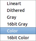
Scan mode: The available scan modes are shown in Figure 19-11 and discussed in the following section.
Scanning resolution: Set this manually or from the menu if you’ve checked the SHOW RESOLUTION LIST box on the VIEW menu. For more information on how to choose the best scanning resolution for your needs, see Scanning Resolutions.
Size of the scanned image in pixels and MB.
Size of the scanned image in a variety of measurement units (centimeters is shown).
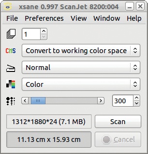
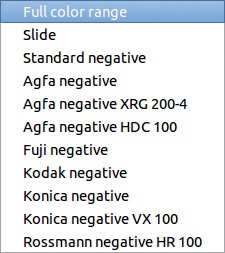
If color management is not enabled in the Preferences menu, the Control window will contain all the entries shown in Figure 19-4. The entry below the scan mode allows you to choose the source medium type. The choices are shown in Figure 19-12. As you can see, specific settings are listed for many types of negatives. FULL COLOR RANGE is the only choice for positives.
The rest of the Control window, between the source medium type and the image size, is covered in Color Handling.
As shown in Figure 19-11, six scan modes are available in the XSane Control window. The last four are the most useful for GIMP users. You can choose between a color or grayscale image and between depths of 8 or 16 bits. The scan mode selected affects the size of the resulting file, and it affects what you can do to the file in GIMP.
With an 8-bit depth, you have 256 possible gray values or 2563 colors. XSane has the capability to scan in 16-bit depth, which results in 65,536 gray values or 65, 5363 colors. Presently GIMP cannot handle 16-bit depth, but plans are to change that in version 2.10 or 3.0. For most users, 8-bit depth is plenty. The human eye is unable to distinguish 65,536 shades of gray, and most monitors and printers are only able to handle up to 8-bit depth images.


That’s not to say that 16-bit depth is completely pointless. If you happen to reduce the output levels range of a gradient (Figure 19-13) dramatically with the Levels tool, you get an almost uniform gray (Figure 19-14). If you then enlarge the resulting narrow histogram to the full range, with an 8-bit depth image, you see stripes (Figure 19-15), whereas with a 16-bit image, you once again have a smooth gradient.


Reducing the output range severely restricts the number of different values. We show the effect on the image in Figure 19-16. First, open the Levels dialog. As shown in Figure 19-17, reduce the output range to the 31 values between 120 and 150. The result appears in Figure 19-18.
Then open the Levels dialog again, and this time enlarge the input range by using only the values between 120 and 150 (Figure 19-19). The 31 values that remain in the image are spread across the 256 possible values, as shown in Figure 19-20. The result is rather ugly because the image has too few values. The effect is especially apparent in the sky. If this image had a 16-bit value range, the effect wouldn’t be noticeable.

You may be wondering why you would ever want to reduce and then enlarge an image’s value range. In reality, you probably won’t ever do that, but it does demonstrate that 16-bit depth can make a difference. The impact is important for high-level photograph handling, and that category of users is waiting impatiently for GIMP to include 16-bit depth.
The LINEART scan mode applies an effect that GIMP can also do and can probably do better. The image is scanned in grayscale, and then a threshold is applied for generating the line art. In GIMP, you can do this with the Image: Colors > Threshold tool, presented in Chapter 12.
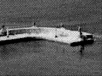
The DITHERED scan mode results in a dithered grayscale image, which was, many years ago, the required format for newspaper printing (see Figure 19-21).

Which scanning resolution you choose depends on the size of the image being scanned, the capabilities of your computer, and what you intend to use the resulting image for.
The available resolutions depend on your scanner and may differ from those shown in Figure 19-22. The lowest ones are available for every scanner, but the highest resolution may be 2400 pixels per inch or less for a low-cost scanner model (like those found on all-in-one printers). For more discussion of scanning resolutions and hardware, see Scanners and Drivers.
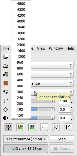
Olivier’s scanner bed is legal sized (8.5 inches × 14 inches). If the definition is set to 300 ppi, the resulting image is 2552 × 4205 pixels, or 31.4MB if the color depth is 8 bits. If the resolution is 4800 ppi and the color depth is 16 bits, the resulting image is 40, 818 × 67, 276 pixels, or 16,090MB, or 16GB. Obviously, 16GB is far too large for today’s personal computers, and that resolution is overkill for the vast majority of users anyway.
Let’s consider image resolution in another way. If you want to put an image on a web page, the final resolution should be 96 ppi. If you want to print it, the resolution should be 300 ppi for normal-quality printing or 1200 ppi or greater for high-quality photo printing. Since the final resolution depends on what the image will be used for, you should have a goal in mind when choosing the scanning resolution. Choose a resolution that’s a little higher than you need. You can scale it down at the very end of the process.
For example, let’s say we have a 4 × 6 inch photograph that we want to publish on a website, with a maximum size of 1024 × 768 pixels. In the XSane Control window, the image’s pixel size is updated when the scanning resolution is changed. Using trial and error, we determine that 192 ppi would be enough. But if we round up to 300 ppi, we have some wiggle room. If the photograph was printed recently, it was probably printed at 300 ppi, so that’s the highest resolution we can actually get. If the photo was printed in the traditional way (in a darkroom), a better resolution is possible. But for this example, 300 ppi is plenty.
Here’s a second example: Let’s imagine we have a 24 × 36 mm film negative and we want to make a high-quality print of the photograph— 1200 ppi in 4×6 inch format. The scanned image will need to be about 4700 × 7000 pixels. In the Control window, we see that the best resolution possible with our scanner, 4800 ppi, is not quite enough.
If this happens, don’t worry. You can get good results by using interpolation to enlarge an image, as long as you don’t overdo it.
In the next section of the Control window, below the settings for scanning resolution, you find a series of parameters for color handling. By default, the dialog has three sliders: one for the gamma value, one for brightness, and one for contrast.
Basically, the gamma value measures the brightness of the median values of the image. If the gamma value is set to 1, the image remains in its original state. If gamma is greater than 1, the image is lighter. If gamma is less than 1, the image is darker. This is also the case when we move the gamma triangle in the Levels tool dialog (see Levels).
Brightness measures the intensity of light in each pixel. Intuitively, increasing the brightness makes an image lighter, and decreasing brightness makes it darker.
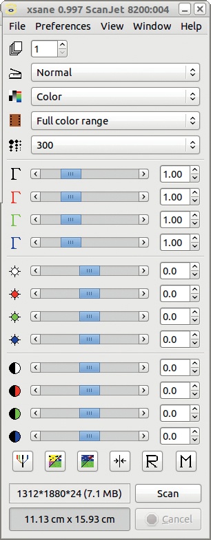
Contrast may be loosely defined as a ratio of the brightness of the lightest pixels to the brightness of the darkest pixels in an image. When contrast increases, the lightest parts of the image grow lighter and more saturated, while the darkest parts grow darker and blacker. Although you can adjust brightness and contrast in XSane when scanning, you have more control in GIMP with the Image: Colors > Brightness-Contrast tool (see Chapter 12) or, better yet, with the Levels tool.
If you click the leftmost button in the bottom row of buttons in the XSane Control window (Figure 19-4), the window expands, as shown in Figure 19-23. The expanded window contains settings for gamma, brightness, and contrast in each of the four channels: Value, Red, Green, and Blue. Making adjustments with these controls can be difficult and tedious, so we recommend ignoring them and using the equivalent tools found in GIMP instead. Also, all changes to brightness and contrast that you make in the Control window are done automatically for all scans until you change the parameters again. Additionally, if you make adjustments in XSane, you won’t see the raw result created by the scanner. You’ll see the scan only after it’s been adjusted.
To summarize, we recommend using XSane simply as a means to scan images. Transformations, such as changes in brightness or contrast, can and should be done in GIMP rather than in XSane. Note that after you acquire the preview, the Control window automatically sets the autoadjust parameters. If you want to use only GIMP for these adjustments, choose SET DEFAULT ENHANCEMENT VALUES by clicking the fourth button in the row of six at the bottom of the Control window.
The following buttons are also found in the bottom row (from left to right):
RGB DEFAULT (
 ): Toggles the size of the Control window, which you can use to adjust gamma, brightness, and contrast values in the Value, Red, Green, and Blue channels.
AUTO ADJUST (
 ): Automatically adjusts the gamma, brightness, and contrast values.
SET DEFAULT ENHANCEMENT VALUES (
 ): Sets gamma to 1.0 and brightness and contrast to 0.
RESTORE (
 ): Restores the enhancement values as set in the preferences.
STORE (
 ): Stores the current enhancement values in the preferences.