
The Render menu contains three submenus and seven normal entries. All the filters in the Render menu replace the current layer or selection with a pattern, and they are generally used on an empty image or an empty layer.
The Clouds submenu contains four filters for generating cloud-like effects, but the first filter is almost exactly the same as the fourth one. We omit Fog, which does not seem very useful.
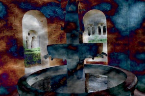
Difference Clouds first generates Solid Noise, which will be discussed below. This filter acts on a new layer, then puts this new layer in Difference mode and merges it with the original layer. We used this filter on the image shown in Figure 17-222 and got the result shown in Figure 17-223.
Plasma generates a colorful, opaque cloud that fills the current layer or the selection. It can be used to generate textures or to add wild colors to a desaturated layer.
The dialog, shown in Figure 17-224, contains randomization parameters that are similar to those of a number of other filters. The NEW SEED button allows you to generate random patterns until you find an interesting one. TURBULENCE [0.1 to 7] controls the smoothness and complexity of the pattern.

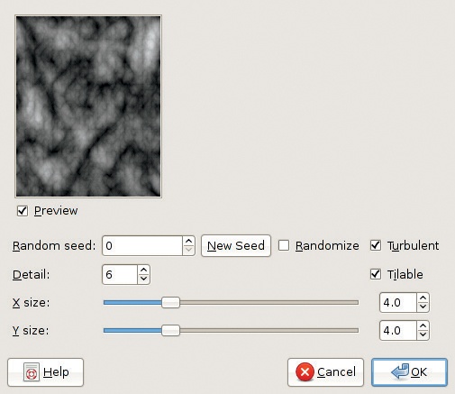
Solid Noise is very similar to Plasma, but it generates a grayscale image and has more settings. It is often used as a way to generate displacement maps or embossing maps.
The dialog, shown in Figure 17-225, begins with randomization settings. The rest of the parameters can be used to modify the generated pattern. TURBULENT makes it rougher. TILABLE makes it tilable. DETAIL [1 to 15] changes the pattern from cloud-like to gravel-like. XSIZE and YSIZE [0.1 to 16] set the level of detail in each dimension.
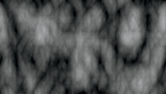
An example is shown in Figure 17-226.
The Nature submenu contains only two entries, but they correspond to powerful and complicated filters.
Flame can be used to generate an infinite array of patterns, including some extraordinary fractals. Almost every attempt leads to compelling computer-generated art, but it is extremely difficult to predict the result, which can be frustrating. Flame paints on the current layer, which means that it can be used several times to generate combinations of successive patterns. If the layer has an Alpha channel, the filter makes the layer transparent before applying the flame pattern so that the current layer disappears and the flames appear on the layer beneath.
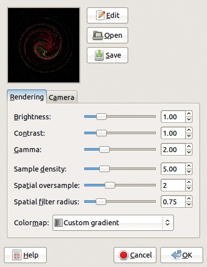
The dialog, shown in Figure 17-227, contains two tabs and a preview window. Next to the preview window are three important buttons. SAVE and OPEN allow you to save and restore a set of parameters that previously generated an interesting pattern.
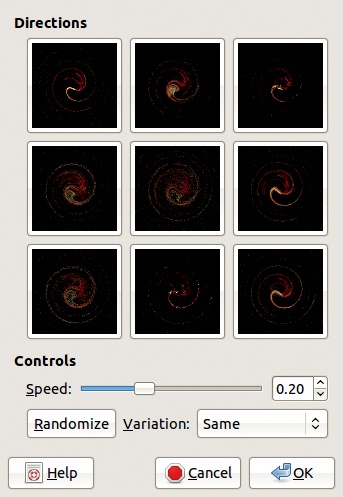
EDIT brings up a new window (Figure 17-228) in which nine variants of the current pattern are displayed. The current one is in the center. Clicking any of the patterns makes that pattern current and generates a new set of patterns around it. SPEED changes the pattern in a way that only the author of the filter fully understands. VARIATION offers 32 fractal themes. RANDOMIZE generates a new set of patterns with the same parameters.
Now switch back to the Rendering tab. The first three settings have an effect that’s apparent in the preview and alter the general color properties of the pattern. The COLORMAP menu changes the color scheme of the pattern. There are six predefined colormaps to choose from. The current gradient is selected by default and is called CUSTOM GRADIENT. The other choices are based on all of the images previously open in this session of GIMP. The other three settings do not have a visible effect in the preview, and to use them with intention you need to understand the mathematics behind the filter (see http://flam3.com/).
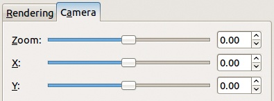
The Camera tab (Figure 17-229) contains only three settings, and these settings change only the preview. The most useful is ZOOM [–4 to +4], which lets you look at the pattern from different distances. The X and Y settings [–2 to +2] move the pattern in the workspace.
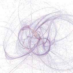
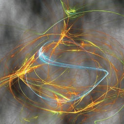
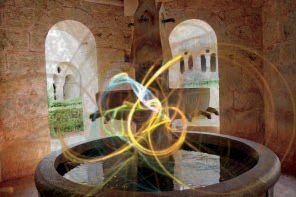
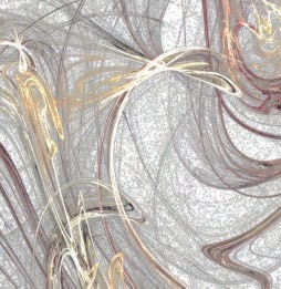
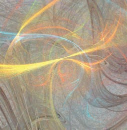
Figure 17-230 to Figure 17-234 show five different examples of results that can be achieved with the Flame filter. The second and third examples (Figure 17-231 and Figure 17-232) show the Flame layered over images from earlier in this chapter, while the fourth and fifth examples (Figure 17-233 and Figure 17-234) resulted from multiple applications of the filter.
IFS Fractal (IFS means Iterated Function System) is even more complicated and difficult to master than the Flame filter. However, with some practice, it is possible to use the filter with some goal in mind and to produce a result that’s reasonably similar to the intended result.
The dialog of the filter (Figure 17-235) contains two sections on top and two tabs on the bottom. The upper-left window shows the geometric figures used to generate the fractal, and the upper-right window shows the result. Initially there are three triangles in the left window, arranged into a larger triangle, and the right window displays what is called a Sierpinsky triangle. On the left, the geometric object (a triangle to start) that is selected is emphasized in boldface. Clicking an object selects it.

The 10 buttons in the top row of the dialog have the following functions:
Move the selected object. The other objects will also move and be deformed when any one object is moved, and the fractal pattern on the right will change as well.
Rotate and scale. Unlike Move, this operates only on the selected object. To rotate an object, select it and move the mouse in a circle centered on that object. To change the size of an object, move the mouse perpendicular to the object’s center. A larger object has more influence on the fractal pattern.
Extend and deform. The effect of this operation can be difficult to control, especially if the mouse pointer is too close to the object center. It’s best to click near the edges of the object. While the object can take on many shapes, its perimeter is constant during this operation.
Create a new object. This operation adds a new object in the center of the left window. As soon as this has been moved, all of the objects, including the one in the preview on the right, will gain a side. If they’re triangles, they become deformed rectangles. Thus if there are five objects, they will all be irregular pentagons. Note that if you add an object immediately after adding the previous one, only this last object will add sides to all the objects when moved. Thus, you could have five irregular rectangles, for example.
Delete the selected object.
Undo the last operation.
Redo the last operation.
Select all the objects. This may be used before any transformation, such as moving or rotating, to allow you to move or rotate all of the objects at once.
Recompute center.

The last button of the top row brings up the IFS Fractal Render options dialog (Figure 17-236), which contains four options. MAX. MEMORY can speed up rendering time, which is especially important if you’re using a large spot radius or a lot of iterations. A high value for MAX.MEMORY can make the computation faster. The number of iterations is the number of times the fractal will repeat. SUBDIVIDE also affects the level of detail, and a high value can lead to a longer computation time. SPOT RADIUS is like a brush size: A large one corresponds to a large brush, while a small one leads to a fractal pattern that is a cloud of small points.
The Spatial Transformation tab displays the parameters of the current object (a triangle at first) as numbers, which can be adjusted directly or by pressing the up or down buttons to the right of each one.
The RELATIVE PROBABILITY slider in the bottom of the dialog sets the degree of influence that the selected object has on the whole pattern.
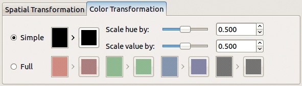
The Color Transformation tab (Figure 17-237) can be used to add color to the fractal pattern. By default, the pattern is generated using the current foreground color. The changes made in the Color Transformation tab are applied to the selected object. SIMPLE changes the object’s color to a chosen color, with settable scales for its hue and value components. FULL allows you to choose a specific color for each of the three RGB components and for the Alpha channel, which is displayed in black.
The best way to learn to use the IFS Fractal filter is to experiment with moving and deforming the three initial objects. Mouse movements should be very precise, since a small movement has a large effect. A tablet and stylus is preferable. Once you’ve found a pattern that you like, you can add a new object to make the pattern richer. Generally, it’s not a good idea to add too many objects, but it’s hard to say exactly how many is too many. Add the color once the pattern is complete. Figure 17-238 is a simple example of an IFS fractal pattern. The filter was used twice on the same layer.
The Pattern submenu contains eight entries for building patterns, some completely predefined, others generated from a large combination of parameters and randomization.

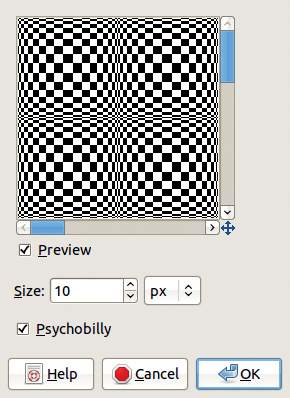
Checkerboard is a very simple filter. It fills the current layer with a regular checkerboard or a distorted one, depending on the settings.
Figure 17-239 shows the dialog of the filter. The SIZE of the squares can be set in a number of different units. Figure 17-240 shows the distorted result of Checkerboard when the PSYCHOBILLY box is checked.
CML (Coupled-Map Lattice) Explorer, the king of all pattern filters, is a very complex tool, difficult to understand and master. It relies on a mathematical model called a cellular automaton.
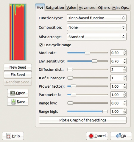
In the top left of the dialog (Figure 17-241) is a long, rectangular preview of the filter result, which does not reflect the shape of the current layer. Below are buttons for altering the randomization: requesting a new seed and switching between a fixed seed or a random one. Below that are buttons for saving the current configuration of parameters and opening a previously saved configuration. The filter dialog also contains six tabs, summarized briefly next.
The filter works in the HSV space, and the Hue, Saturation, and Value tabs contain the same set of parameters, but changes are applied only to the specified component. Next we’ll walk through the components that are common to all three tabs.
FUNCTION TYPE includes the list of options and functions shown in Figure 17-242. The corresponding parameter (Value, Saturation, or Hue) can be taken from the image; be standard cyan; or be computed using one of the functions, which may use a parameter k, specified below in the dialog, or a power factor p, also specified below.

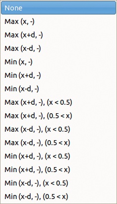
The COMPOSITION function can be chosen from the list shown in Figure 17-243. An entire book could be written about the theory behind and effect of these functions, but this is not that book, so we simply suggest that you experiment with the various functions.
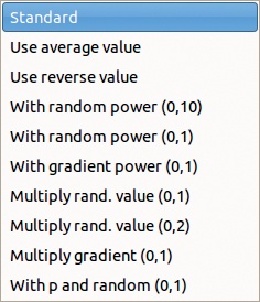
MISC ARRANGE also contains a list of functions, shown in Figure 17-244. As with COMPOSITION, the effect of these functions is difficult to explain. Below MISC ARRANGE, the tab contains a checkbox and a lot of sliders. The best way to understand their purpose is to try them out.
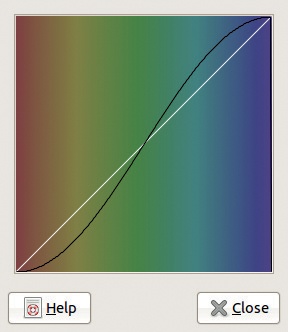
The PLOT A GRAPH OF THE SETTINGS button displays the graph shown in Figure 17-245. This graph provides a visual display of the settings and may help you to better understand the influence of the different functions.
The Advanced tab is shown in Figure 17-246. It contains three sliders for each component of the HSV model. The MUTATION RATE affects the changes to a pixel relative to its neighbors. Experimentation is again the best way to understand what effect changes will have.

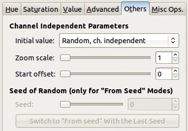
The Others tab is shown in Figure 17-247. The INITIAL VALUE field contains the menu shown in Figure 17-248, which allows you to choose the initial value and includes several methods of selecting random sources in addition to fixed values such as black or white. The random seed can be changed with the lower slider. The ZOOM SCALE slider lets you look more closely at the pattern, but zooming in too far can lead to a strong pixelation effect.
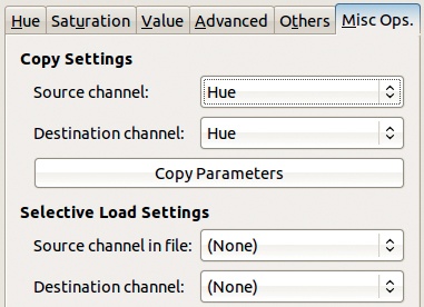
The Misc Ops. tab (Figure 17-249) lets you copy the parameters from one of the HSV channels to another. The two parameters at the bottom change the effect of the OPEN button, on the left of the dialog. They allow you to load only one channel from the source file and to put the parameter values from one channel into a different channel.

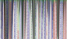
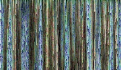
The number of possible combinations of the different functions in the CML Explorer is huge, and with the addition of the parameters, the number of possible results is incredibly vast. The name of the filter, CML Explorer, reflects the fact that the best way to use this tool is to explore the innumerable capabilities of the CML algorithm. Figure 17-250 to Figure 17-253 show just a few random examples of the results it can produce. Readers are strongly encouraged to explore the filter for themselves.


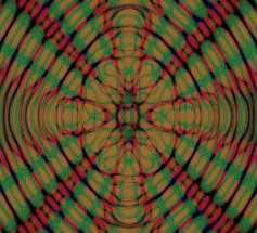
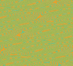
Diffraction Patterns creates wave interference patterns from an image. The authors of the filter never wrote an explanation for the function of the parameters, so the only way to learn what they do is to experiment. The preview is rather small and doesn’t update automatically. To update it, click the PREVIEW! button.
The dialog, shown in Figure 17-254, contains four tabs. However, the first three are identical. Each contains three sliders [0 to 20] for the three components of the RGB model. The tabs alter the frequencies, contours, and sharp edges. The last tab contains options for BRIGHTNESS [0 to 1], SCATTERING [0 to 100], and POLARIZATION [–1 to 1].

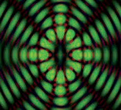

Diffraction Patterns inevitably yields an interesting result, but it is very difficult to predict what the result of changes to any one parameter will be. Figure 17-255 to Figure 17-257 show three examples.
Grid simply draws a grid on the current layer. The dialog, shown in Figure 17-258, allows you to set the parameters separately for the horizontal lines, the vertical lines, and the intersections.

It’s possible to generate intersections that are thinner or thicker than the lines themselves. These intersections look like plus signs. You can set the following parameters:
The width of the lines, including the arms of the intersection plus signs.
The spacing of the lines. For intersections, this clears the space between the line crossing and the plus sign arms. If this is confusing, try it out and see the effect for yourself.
The offset of the lines with regard to the upper-left corner. For the intersections, this is the length of the plus sign arms.
The color of the lines or intersections.
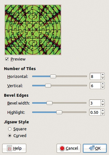
Jigsaw draws the pieces of a very uniform jigsaw puzzle on the current layer.
The dialog, shown in Figure 17-259, allows you to specify the number of tiles in the horizontal and vertical directions. The relief effect can be adjusted by changing the BEVEL WIDTH [0 to 10] and the HIGHLIGHT [0 to 1]. Finally, the tiles can either have sharp edges or be slightly curved. The result is shown in Figure 17-260.
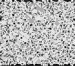
The Maze filter creates a maze that fills the current layer. The walls are black, and the paths are white.

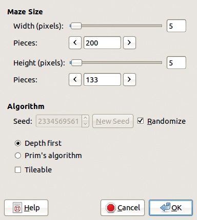
The dialog, shown in Figure 17-261, allows you to choose the width of the paths and the number of paths, horizontally and vertically. The maze generally looks best when the width and height are equal. The number of paths (called number of pieces) is linked to the width and height. The maze can be completely randomized, or you can set a seed or generate one with the corresponding button. There are two algorithms that can be used to generate the maze, and the result can be made tilable, in which case the maze extends to the boundaries of the layer. Otherwise, there is a white frame around it.
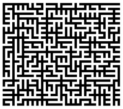
Our result is shown in Figure 17-262.
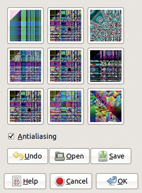
Qbist is a random texture generator.
The dialog shown in Figure 17-263 is simple. Nine patterns are generated at the same time. The center one is the current selection, and the eight surrounding patterns are random variations on that selected pattern. If you click any of the nine patterns, that pattern becomes the new center pattern, and eight new derivative patterns are generated. Clicking the center pattern does not change it, but new derivative patterns are generated. There is no way to control the generation, since the patterns that appear are a matter of random chance. Although you can’t intentionally generate a pattern again, you can save an interesting pattern and reload it later. It is also possible to undo the generation process and return to a previous set of patterns.
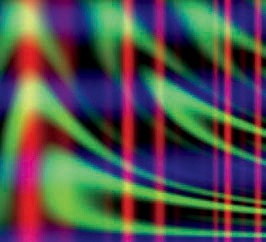

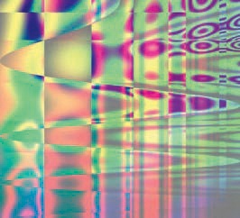
Figure 17-264 to Figure 17-266 show three random examples of Qbist-generated patterns.
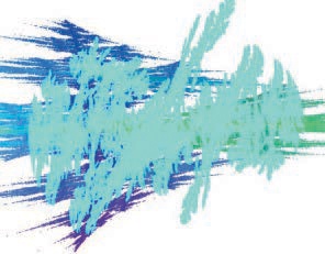
Sinus is yet another texture generator. It uses two colors to create wave-like patterns using the mathematical function sine. The texture fills the current layer.

The dialog, shown in Figure 17-267, contains three tabs. In the Settings tab, XSCALE and Y SCALE [0.0001 to 100] set the number of curves in the X and Y directions. The higher the value, the more compressed the curve is. COMPLEXITY controls how the two colors are combined. The randomization is similar to that of other filters. The FORCE TILING? checkbox allows you to make the texture tilable. Finally, an IDEAL texture is more symmetrical than a DISTORTED texture.
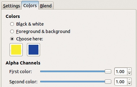
The Colors tab (Figure 17-268) allows you to choose the two colors, which can be set to black and white or the current foreground and background colors, or they can be chosen using the Color chooser. Two sliders can be used to make these colors semitransparent if the layer has an Alpha channel.
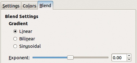
The Blend tab (Figure 17-269) contains a selection of three function types that determine the shape of the waves. The EXPONENT slider sets the respective weight of the two colors.
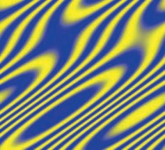
Two examples of patterns generated with Sinus are shown in Figure 17-270 and Figure 17-271.
Circuit builds a maze that looks like a jumble of curved roads or a plate of spaghetti. It also vaguely resembles a diagram of circuitry, hence its name.
The dialog does not contain many parameters. The filter generates a maze and then oilifies it. The settings include the mask size for the Oilify filter and a randomization seed, which allows the filter to generate a unique maze each time it’s used. The width of the paths and the number of walls cannot be set. When the SEPARATE LAYER checkbox is checked, the circuit will be created on a new layer. If there is a selection, the circuit is generated within the selection, and a checkbox allows you to keep the selection active after the filter operates. Finally, if the NO BACKGROUND box is checked, the intervals between the paths are transparent, and the remaining selection excludes these transparent parts.
The result of Circuit is shown in Figure 17-272.
Fractal Explorer is a fractal generator that’s much simpler than the IFS Fractal filter. Its most interesting feature is the long list of available predefined fractals.
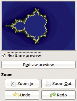
The dialog is unusually wide, so only the left side, which is common to all tabs, is shown in Figure 17-273, while the first of the three tabs, Parameters, is shown in Figure 17-274.
The left side of the dialog contains a large preview, a checkbox that turns the automatic update on or off, and a button that can be used to manually update the preview. Below that are buttons to zoom in or out and buttons to undo or redo changes in the zoom. ZOOM IN and ZOOM OUT zoom by a predefined amount. You can click and drag in the preview window to create a new viewing rectangle, which will zoom in on a specific part of the fractal.

In the Parameters tab, skip down to the bottom and begin by choosing a FRACTAL TYPE. (If you’ve used this filter before, click the RESET button first.) The appearance of a fractal strongly depends on the number of ITERATIONS [1 to 1000], set using the corresponding slider. The BARNSLEY 1 fractal is invisible unless you zoom out. The BARNSLEY 2, SPIDER, MAN’O’WAR, and SIERPINSKI become invisible if the number of iterations is greater than 50. On the other hand, a very large number of iterations can enhance the MANDELBROT fractal, which then has a great depth of detail that you can zoom in on.
The other parameters change the aspect and form of the fractals. The CX and CY sliders have a dramatic effect on the aspect, except with MANDELBROT and SIERPINSKI. The four direction parameters simulate rotating a plane on which the fractal is drawn.
The SAVE and OPEN buttons allow you to save an interesting combination of parameters for use later.
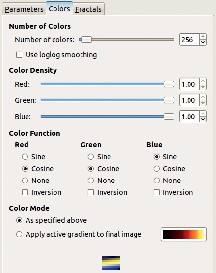
The Colors tab (Figure 17-275) allows you to adjust the appearance of a fractal. A gradient at the bottom of the tab shows the available colors, which change as the NUMBER OF COLORS slider is changed. The COLOR DENSITY sliders do not change what colors are available but how colors are used in the fractal. The COLOR FUNCTION radio buttons, along with the INVERSION check-boxes, also change how the available colors are applied. The color gradient (which changes the available colors) can be replaced using the COLOR MODE radio buttons along with the large gradient selection button.
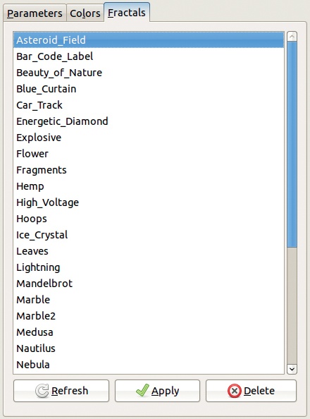
The Fractals tab (Figure 17-276) is simply a list of 33 predefined fractals. When you choose one of them and click the APPLY button, the two other tabs change to reflect the corresponding parameters. You can subsequently change some of the parameters to personalize the fractal.
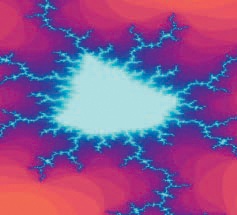
As is the case with other render filters, this filter is the source of endless experiments. Three example fractals are shown in Figure 17-277 through Figure 17-279.
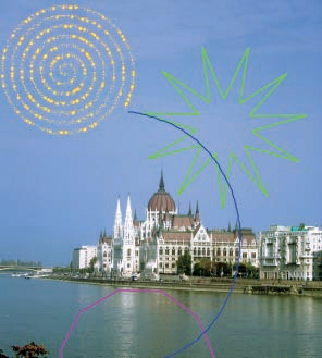
Gfig is something special within the framework of GIMP. It is not really a filter but rather a tool to create geometric figures. Although GIMP is intended to create raster or pixelized images, Gfig works like a vector graphics tool, but the graphics it creates are pixelized. They are created in a new layer, on top of the source image.


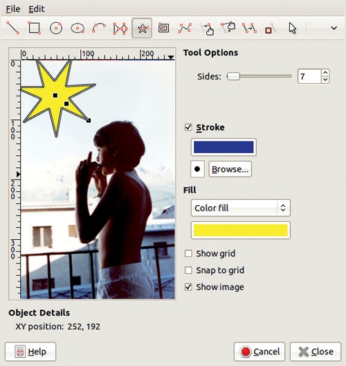
The dialog, shown in Figure 17-280, shows the initial image. We chose a dark blue as the stroke color and a vivid yellow as the fill color, and we drew a regular star heptagon using the Star tool, selected from the bar at the top of the dialog.
The preview shows the entire initial image, zoomed out to fit the dialog size. The preview size cannot be changed. The top bar contains buttons for 21 tools, of which only the first 14 are shown here. The remaining 7 can be accessed using the drop-down menu on the far right. Most of the tools have no options. However, the Star tool does have a slider for adjusting the number of sides that the polygon will have.
The geometric figures created using the first nine tools in the bar (from left to right) can be stroked and filled. Stroking is done using the selected color and brush, which can be changed by clicking the relevant buttons. Filling can be done with a color, pattern, shape gradient, vertical gradient, or horizontal gradient. The color, the pattern, or the gradient can be changed using a button that appears just below the field.
Note that there is no way to change the scale of the brush, so to adjust the brush, you must have a collection of brushes of different sizes. There is one in the brush folder, in a subfolder called gimp-obsolete-files. Since this subfolder is not visible from the Brushes dialog, you must copy all the brushes it contains to your own brush folder. Place them in a subfolder called Obsolete, so they all automatically bear the corresponding tag. See Chapter 22 for more details about the location of the brush folder.
Three checkboxes can be used to do the following:
Show a regular grid.
Snap to this grid.
Show the image (i.e., preview the result of the filter).
This filter has its own menus, which replace the general GIMP image menus, making this filter very different from any other. The File menu contains three entries:
The Edit menu contains four entries:
UNDO (
 ) undoes the last action. However, there is no redo provision.
CLEAR deletes the current drawing. This can be undone.
GRID (
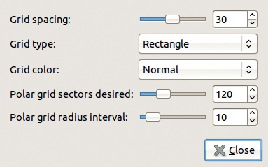
 ) opens the dialog shown in Figure 17-281, where you can set the characteristics of the grid:
PREFERENCES (
 ) opens the dialog shown in Figure 17-282. There are three checkboxes that show the mouse position (in OBJECT DETAILS), show control points in the image, and turn on antialiasing. You can also set the maximum number of undo [1 to 10], and you can choose whether the background is transparent, the foreground or background color, white, or a copy of the image. A checkbox can be used to feather the drawing, with a radius set by the slider [0 to 100].

You can create several geometric shapes in the drawing, but when you add a new form, build it first and then change its stroke and fill parameters, or the changes will affect the previous shape.
The object-creating tools, corresponding to buttons in the top bar, are as follows:
Line: Click the origin and drag to the end. This creates a straight line.
Rectangle: Click one corner and drag to the opposite corner.
Circle: Click the center and drag to the radius.
Ellipse: Click the center and drag to the corner of the embedding rectangle.
Arc: Click the three points defining the arc.
Regular polygon: Set the number of sides [3 to 200], click the center, and drag to one of the vertices.
Star: Works like the Regular polygon tool.
Spiral: Set the number of turns [1 to 20], the orientation (right or left), and then click and drag as with the Circle tool.
Bézier curve: Click the successive control points and
 -click the final one. The options allow you to close the curve and to show the line frame, which is composed of the tangents from the last control point.
The next five buttons can be used to make adjustments to the shapes you’ve drawn. First select the shape by clicking one of its control points. Then, depending on which button you’ve selected, you can move the entire shape, move one of the control points, copy the shape, or delete it.
The shapes are superimposed in the order they were built. The additional tools available on the right of the top bar raise or lower the selected shape by one position, put it at the top or the bottom of the stack, display only one object, or show all objects.
Gfig offers a set of operations that allow you to create complicated geometric objects. One example is shown in Figure 17-283, where very precise shapes could be drawn thanks to the large image size (2304 × 3456).
The Lava filter simulates lava as seen in a volcano crater.
The dialog, shown in Figure 17-284, has no preview. You can set the randomization seed, the size of the waves [0 to 100], and the wave roughness [3 to 50]. The gradient determines the colors used in the waves, which can be a nice lava red or something completely unrealistic. If there is a selection in the current layer, you can choose whether to keep it. You can create the lava on a new layer, and you can choose to use the current gradient to color the lava.

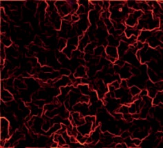
An example made with the Lava filter is shown in Figure 17-285.
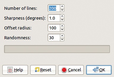
Line Nova draws a multispiked star on the current layer, in the foreground color.
In the dialog, shown in Figure 17-286, only four parameters can be set: the number of spikes (at least 40), their sharpness [0 to 10], the offset radius (the radius of the central circle), and the randomness of the spike lengths.
A star created with Line Nova is shown in Figure 17-287.
Sphere Designer creates a 3D sphere on the current layer, which covers up most of the layer contents.
The dialog, shown in Figure 17-288, contains a preview that is automatically updated. The sphere image is built with several texture layers (which are merged when the sphere is generated). These layers are listed on the top right in the dialog. The dialog also has buttons to create a new layer, duplicate the current one, or delete it. The OPEN and SAVE buttons allow you to save the current settings into a file or to restore a previously saved set.

When a layer is selected, its PROPERTIES can be set. The layer’s TYPE can be TEXTURE, BUMP, or LIGHT, and its TEXTURE can be chosen from the list shown in Figure 17-289. Two color buttons can be used to select colors for TEXTURE type layers. LIGHT type layers only use the first color, while BUMP type layers are colorless.
Four sliders set the characteristic of the texture. SCALE and TURBULENCE [1 to 10] are general settings with effects that depend on the layer type. AMOUNT [0 to 1] sets the influence of the layer on the sphere. EXP [0 to 1] sets the strength of the pattern and affects only the texture types MARBLE, LIZARD, NOISE, and SPIRAL.
The TRANSFORMATIONS section of the dialog contains three groups of sliders, and each group has a slider for the X, Y, and Z coordinates. SCALE [0 to 10] stretches or compresses the pattern in the corresponding direction. ROTATE [0 to 360] rotates the pattern, but not the sphere itself. POSITION [–20 to +20] sets the position of the texture on the sphere, or the position of the light if the layer type is LIGHT.


See Figure 17-290 for an example of a sphere generated with Sphere Designer.
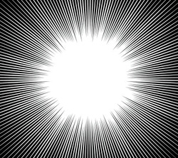
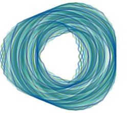
Spyrogimp simulates a spirograph (a geometric drawing toy) on the current layer. Although the concept is fairly simple, there is a wide range of possible results, so this filter can be yet another source of endless experimentation.
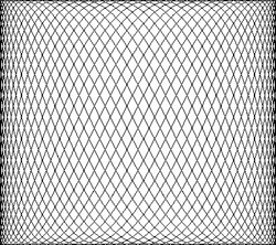
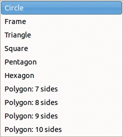
In the dialog, shown in Figure 17-291, the first option is the curve type. Figure 17-292 to Figure 17-294 illustrate the three available types. The parameters mimic the properties of a spirograph, which creates designs using gears with various numbers of teeth [1 to 120] and various shapes (see Figure 17-295). Each design is done using two gears, and the complexity of the design depends on the value of the greatest common multiple of the numbers of teeth. The combination of 120 and 60 leads to a very simple curve, while 120 and 61 yield an extremely complex curve, with a moiré effect. The most complicated design in the given range occurs when the gears with 120 and 119 teeth are used. More complicated designs take longer to render.
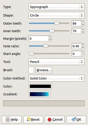


MARGIN sets the width of the border of the image, where the design is not drawn. It can be negative, which causes the design to extend beyond the edges of the image. HOLE RATIO sets the diameter of the center hole. START ANGLE sets the angle of the first line that’s drawn, which is not very important since the design is circular and closed. Changing the START ANGLE just rotates the design.
The TOOL option can be used to select among Pencil, Brush, or Airbrush. The Brush works best when a very small diameter is used. See Gfig for more information on adjusting the brush size. The COLOR METHOD can be a solid color or a gradient with a repeated sawtooth or triangle pattern. The color or gradient can be changed using the buttons below the COLOR METHOD menu.
See Figure 17-296 and Figure 17-297 for examples of designs made with Spyrogimp.