All 10 filters in the Map menu map an image onto an object in order to deform the image; for example, by adding relief to it, curving it, or making it seamless. The map filters often produce very dramatic effects.
Bump Map embosses an image using another image as a map. If the map is smaller than the image, some areas of the image will be left unaltered.
In the dialog, shown in Figure 17-191, the BUMP MAP menu lists all of the images open in GIMP and the images previously open in the same session. MAP TYPE can be set to one of three modes, which determine how the bump height is related to the map image luminosity: linear, spherical, or sinusoidal.
It’s generally advisable to leave the COMPENSATE FOR DARKENING box checked to avoid overly dark results. By default, bright pixels generate bumps, and dark pixels generate hollows; if the INVERT BUMPMAP box is checked, bright pixels will be hollows, and dark pixels will be bumps. When TILE BUMPMAP is checked, the resulting image will be a tilable relief, which can be used as a background for a web page, for example.
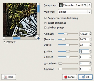

AZIMUTH [0 to 360] sets the direction of the light. ELEVATION [0.5 to 90] sets the position of the light above the horizon (90 means vertical). DEPTH [1 to 65] sets the difference in height between hollows and bumps. XOFFSET [–1000 to +1000] displaces the map horizontally with regard to the image, and YOFFSET displaces it vertically. WATERLEVEL [0 to 255] has an effect only if the image contains transparency: Transparent areas are treated as darker and become hollows (if the bump map is not inverted). If Waterlevel is increased, these hollows progressively disappear. AMBIENT [0 to 255] is the level of ambient light, which reduces the effect of the relief when it’s very high.
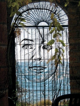
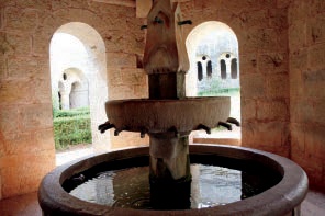
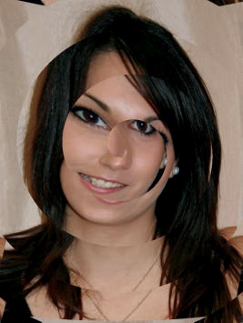
Our result is shown in Figure 17-192. The image itself was used as a map. Figure 17-193 shows the application of the filter to the same image, using the portrait from Figure 5-44 as a map and with slightly increased DEPTH and ELEVATION.
Displace uses two images as displace maps, one for X and the other for Y. These two images must be the same size as the original image, which is being altered. All three images must be open in GIMP when the filter is selected. Only the value component of the map images is used, so it makes no difference whether they’re color or grayscale images.
Most of the options in the dialog, shown in Figure 17-194, deal with displacement. When the DISPLACEMENT MODE is CARTESIAN, the displacement in the target image is calculated by multiplying the chosen displacement value (X or Y) by the value component of the pixel in the map. It’s possible to uncheck one of the dimensions and displace the target image in only one direction. When the displacement mode is POLAR, X is the radial distance (called Pinch) and Y the tangential one (called Whirl). The EDGE BEHAVIOR specifies how the image edges are handled: If the mode is WRAP, the missing pixels are taken from the opposite side; if it is SMEAR, neighboring pixels are duplicated in areas that are missing pixels; if BLACK is chosen, missing pixels are filled with black.
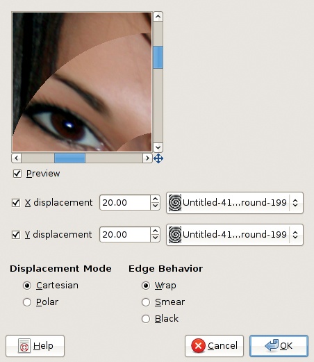
Computing the actual displacement is rather complicated. In the X and Y dimensions, a pixel value in the displace map that’s less than 127 results in a displacement to the left, and a value greater than 127 results in a displacement to the right. In polar displacement, pixels with a value greater than 127 are displaced outward, and pixels with a value less than 127 are moved toward the center of the image.

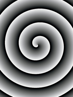
To demonstrate Displace, we built the map shown in Figure 17-195 by creating a new image the same size as the image to be filtered and filling it with a spiral gradient. The result of Displace in CARTESIAN mode is shown in Figure 17-196. Figure 17-197 shows the result of the same filter and parameters, in POLAR mode.
Fractal Trace maps the image to a Mandelbrot fractal.
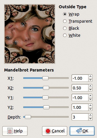
The dialog of Fractal Trace is shown in Figure 17-198. The OUTSIDE TYPE option determines what appears in the area around the original image. Only WRAP produces a fractallike pattern of smaller copies of the image. The other three options, TRANSPARENT, BLACK, and WHITE, replace the background with transparency, black, or white. The MANDELBROT PARAMETERS sliders are sensitive and should be set with care, especially the DEPTH: At high values (the maximum is 50), the initial image is unrecognizable.
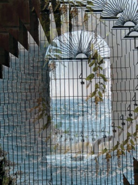
The result of Fractal Trace is shown in Figure 17-199.
Illusion doesn’t use a second image as a map. Instead, it uses multiple copies of the image itself, at various sizes, orientations, and levels of brightness, to build something like a kaleidoscope image.

There are only two adjustable parameters in the dialog: the number of copies of the image [–32 to +64] (a negative value inverts the rotation direction) and the mode.
The result is shown in Figure 17-200.
Make Seamless has no dialog and no options. It transforms the image to make it tilable. To achieve this, it cuts a copy of the image into quarters, puts each quarter in the corner opposite to its original position, and creates a smooth transition with the original image.
Our result is shown in Figure 17-201.
Map Object maps one or more images onto a plane, a sphere, a box, or a cylinder. The light source, the material properties, and the orientation of the object can be adjusted.
The dialog of the filter contains four or five different tabs, depending on the objects chosen. The Options tab appears in Figure 17-202, along with the preview. There are zoom buttons, as well as a PREVIEW! button, which is useless in the Options tab but is useful in the other tabs. The SHOW WIREFRAME checkbox, if checked, adds a wireframe of the object to the preview.
The MAP TO option in the orientation tab allows you to choose among the four different objects. There are also checkboxes to replace the background with transparency and to create a new image. Another works only for a plane: TILE SOURCE IMAGE fills the area of the image that is left empty with the content that was pushed off the opposite side.
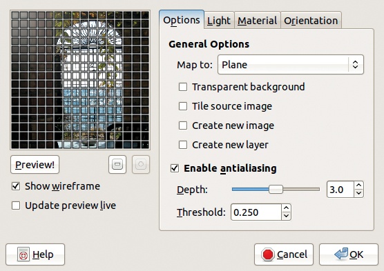

ENABLE ANTIALIASING should generally be left checked, and the corresponding slider and counter can also be left as they are.
In the Light tab (Figure 17-203), the LIGHT-SOURCE TYPE can be set as a point, as directional lighting, or as no light at all. The three coordinates determine the POSITION of the point of light or the DIRECTION VECTOR for directional light. LIGHTSOURCE COLOR brings up the Color chooser.
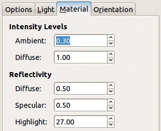
In the Material tab (Figure 17-204), the INTENSITY LEVELS change the properties of the indirect (AMBIENT) or the direct (DIFFUSE) light. On the default setting, areas that aren’t directly lighted are very dark. The REFLECTIVITY of the object is specified by three parameters: DIFFUSE sets the brightness of reflecting parts, SPECULAR the intensity of the highlights, and HIGHLIGHT changes the precision of the highlights. These parameters can be difficult to set properly, and the PREVIEW! button really comes in handy.
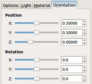
The Orientation tab (Figure 17-205) contains a couple of three-dimensional coordinate sliders, which set the position and rotation of the object. The origin (0,0) is always the top-left corner of the object. The position coordinates have the range [–1 to +2], and the rotation coordinates have the range [–180 to +180]. The PREVIEW! button should be used regularly to check the new object position, since it is very difficult to accurately predict the effect of these sliders.
The Box tab (Figure 17-206) is present only if the object is a box. The tab is mainly used to choose images that will be mapped to the six faces of the box. The images must be open in GIMP when the filter is selected, and they’re automatically scaled to fit on the box. The three sliders [0 to 5] change the size of the box edges.
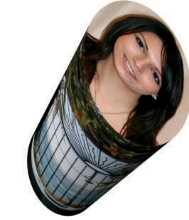
The Cylinder tab (Figure 17-207) is present only if the object is a cylinder. It allows you to choose the images that will be mapped to the cap faces of the cylinder. The image on the curved face of the cylinder is always the current image. The two size sliders [0 to 2] can be used to change the dimensions of the cylinder.
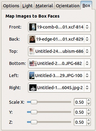

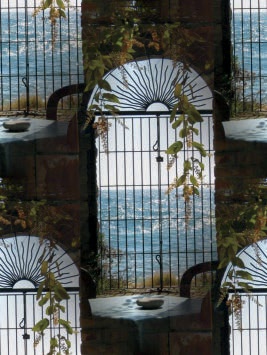
Figure 17-208 through Figure 17-211 show examples of the Map Object filter mapping some of our sample images to a box, a cylinder, a sphere, and a plane, respectively.
Paper Tile cuts the image into many squares of the same size and moves them around randomly, leaving small spaces between some and overlapping others.
In the dialog, shown in Figure 17-212, you can set the size of the squares and the number of squares in the horizontal and vertical directions. These parameters are linked: Setting the X and Y parameters automatically changes the WIDTH and HEIGHT, and vice versa. MOVEMENT is randomly computed within a percentage limit of the size. If pixels are shifted out of the image, they can be simply cut, or they can be wrapped around the image so that they’ll appear on the other side. FRACTIONAL PIXELS are pixels not covered by any paper squares. They can be filled based on the selected background type (BACKGROUND), left as they are (IGNORE), or cut out (FORCE). BACKGROUND TYPE specifies what is done to the spaces between the paper tiles after they are moved. The space can be transparent; it can contain the original image, as is or inverted; or it can contain the foreground or background color or a different color selected with the Color chooser. The CENTERING box, if checked, gathers the tiles toward the center of the image.


Our result is shown in Figure 17-213.
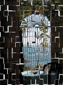
Small Tiles creates smaller duplicates of the image, displayed in a grid.
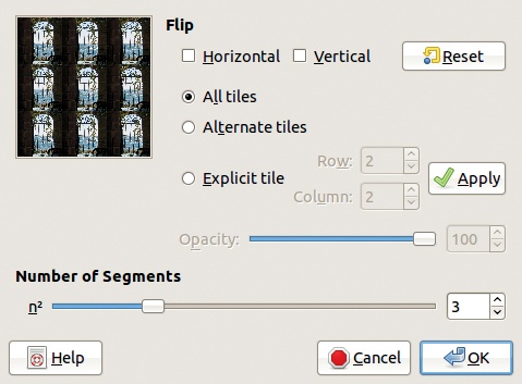
In the dialog, shown in Figure 17-214, the most important setting is the NUMBER OF SEGMENTS (i.e., the number of rows and columns of small images in the resulting image). For example, a value of 3 results in a total of 9 copies. Copies can be flipped, horizontally or vertically or both. The flip can be applied to all tiles, to every other tile, or to an EXPLICIT TILE, which you can specify by its column and row. Finally, if the image layer has an Alpha channel, the OPACITY of the result can be set to less than 100%.

See Figure 17-215 for the result.
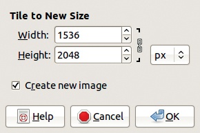
Tile builds an image that contains as many copies of the original image as needed to fit the new size.
The dialog, shown in Figure 17-216, is very simple. The new size of the image can be set using the linked fields, and the change can be applied to the current image or to a new image. If the new size is smaller than the current image, the image will be cropped in the result. If the new size is larger, there will be several copies of the original image tiled in the new image.

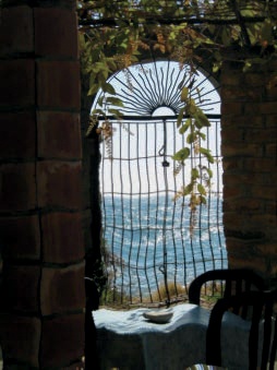
Our result is shown in Figure 17-217. The initial image size was 768 × 1024.
Warp is a complicated filter, and the result is difficult to predict, since there is no preview. The trial-and-error approach is often impractical, as the filter’s processing time is rather long. Warp displaces the pixels of the image according to the gradient slopes of a grayscale displacement map.
The dialog is shown in Figure 17-218. To demonstrate the filter, we built a displacement map by creating a new image, the same size as the original one (Figure 17-139), filled with solid noise (Image: Filters > Render > Clouds > Solid Noise). This displacement map contains gradients in random directions. The STEP SIZE is set to 10 by default, which would result in image pixels being displaced by only 1 pixel. We increased the step size to 100 in this example. The filter effect is repeated the number of ITERATIONS times. The ON EDGES radio buttons do not need explanations. Figure 17-219 shows the result.
The second part of the dialog, ADVANCED OPTIONS, includes the following options:
DITHER SIZE can be used to create a dithered effect, as shown in Figure 17-220. The step size was set to zero, so there was a dithering effect but no displacement.
A MAGNITUDE MAP alters the target image based on the map’s brightness rather than its gradients, and it is used in conjunction with the displacement map to create the final effect. Black regions of the magnitude map cancel the filter effect, while white regions result in the strongest effect. In Figure 17-221, the magnitude map used was a simple vertical gradient from black at the top to white at the bottom, so the effect of the displacement map was strongest at the bottom of the image. The changes are applied some number of times specified by SUBSTEPS.
ROTATION ANGLE is the angle between the displacement and the gradient. In Figure 17-221 it was set to 90.


The third part of the dialog, MORE ADVANCED OPTIONS, allows you to use two additional maps. These maps will have an effect only if the corresponding coefficient is greater than zero.