
The next part of the Image: Colors menu contains four submenus: Auto, Components, Map, and Info. We’ll consider them each in turn.
The Auto submenu is shown in Figure 12-83. It contains tools that have no corresponding dialogs. When selected, they adjust the image instantly, using automatic settings, as the name suggests. Because you can’t customize the settings for these tools, their utility depends on the image being processed. To demonstrate their effects, we have included the Histogram dialog with each demonstration image and with the initial image, which is shown in Figure 12-84.

The Equalize tool automatically adjusts the brightness of all colors, so that each possible brightness value occurs about the same number of times in the image. The histogram for the image in Figure 12-85 shows that the color values that occur most frequently, in this case [0 to 80], are stretched the most: See the flat part in the middle of the histogram. In this example, the result is bizarre and is not an improvement. In other cases, the result may look better.
The White Balance tool operates separately on each of the RGB channels. It removes the least-used pixel values from both ends of the histogram and then stretches the remaining pixels to extend across the full range. In Figure 12-86, the brightest pixels disappeared, and the remaining pixels were stretched along the full range. The picture is much lighter, and this time the result could be considered an improvement.
The Color Enhance tool makes adjustments using the HSV model: It increases the saturation without changing the hue or the value. The effect on this image, shown in Figure 12-87, is rather unpleasant. The Color Enhance tool flattened the histogram without extending the color range. The result is slightly better when we apply the White Balance tool first, but automatic tools such as this one clearly have limitations.


The Normalize tool stretches the brightness of the image so the darkest point is black and the brightest point is as bright as possible in its current hue. To best demonstrate this, we’ll use the image shown in Figure 12-88, which we modified with the Levels tool: We moved the right triangle under INPUT LEVELS to position 212 to remove the few pixels brighter than this value and the right triangle under OUTPUT LEVELS to the same position to retain the same overall brightness in the image. When applied to this modified image, the Normalize tool produces a visible effect (Figure 12-89), which it does only when there are no pixels on the far left or right of the histogram.

The Stretch Contrast tool works the same way as the Normalize tool, but rather than stretching the Value channel, it stretches the RGB channels separately. These two tools result in visibly different effects only if the RGB channel ranges differ significantly, and when the Stretch Contrast tool does produce a unique result, it can generate color distortions. To create Figure 12-90, we began with the same modified example that we used for the Normalize tool, and the result is very similar.
The Stretch HSV tool works the same way as the Stretch Contrast tool, but it operates on the three channels of the HSV model instead of on the three RGB channels. This method can produce a better or worse result, depending on the image. Our result, shown in Figure 12-91, is almost identical to the initial image.


The Components menu is shown in Figure 12-92. Its four tools operate on the RGB channels.
This tool uses the values from all three of the RGB channels to compute new values for each one of them. Initially, each output channel receives only the corresponding input channel. Figure 12-93 shows the Red channel dialog.
At the top of the Channel Mixer dialog is a preview of the image, with zooming and panning enabled. Below that is the OUTPUT CHANNEL selection menu. The next three sliders, which have a range of [–200 to +200], allow you to set the percentage of the corresponding channel that will be assigned to the current output channel. If we change the output channel, we can define another set of percentages.

If we check the MONOCHROME box, the image becomes grayscale, and we can use the sliders to set the proportion of each of the RGB channels that are used to build the monochrome image. For example, when we select Image: Image > Mode > Grayscale, a grayscale image is created using the values 21, 72, and 7 for the three RGB channels, from top to bottom.
The PRESERVE LUMINOSITY checkbox maintains the initial luminosity of each pixel, which prevents the resulting image from being overly bright.
The set of buttons at the bottom of the dialog allow us to save the current settings, reload previously saved settings, and reset everything to the initial values.
You can make very fine adjustments to the colors of an image with this tool, but mastering it is difficult.
The Decompose tool separates the channels of the image into separate grayscale images or layers based on the chosen color model. Its dialog, shown in Figure 12-94, is fairly simple. At the top is the COLOR MODEL menu, and below that are two checkboxes. Checking the first box decomposes the image to layers; otherwise the decomposition results in separate images. The second box is included for CMYK printing purposes. When checked, every pixel that’s part of the current foreground color will be black in the decomposed images or layers. This is commonly used to show crop marks on all channels as a way to aid in alignment.


The available color models, shown in Figure 12-95, are explained next.
RGB: This decomposition allows us to work on the channels separately and then recompose the image. One of the channels can also be used as a mask.
RGBA: Similar to the RGB model, except with this model, an Alpha layer or image is also created for the image’s Alpha channel.
HSV: The layers or images represent the components of the HSV model. The Hue channel is rather compressed, and the result has no natural meaning, as shown in Figure 12-96. The Saturation channel is also not very meaningful (Figure 12-97). In contrast, the Value channel returns an accurate grayscale representation of the image.
HSL: Similar to the HSV model, but the Value channel is replaced with Lightness, which is similar conceptually but calculated a little differently. The calculations for the Saturation channel also differ slightly.
CMY and CMYK: These models are generally used to decompose an image in order to pass it to printing software that requires decomposition.
ALPHA: A new image is created from the Alpha channel of the image. For example, Figure 12-98 was generated from an Alpha channel built with Image: Colors > Color to Alpha, using white as the color.
LAB: The Lab (or L*a*b*) color space includes several models that are intended to be more representative of human vision than the other color models. The L channel represents luminosity, and the A and B channels represent color in the form of opponent color axes. The Lab color space was designed based on the opponent process theory, which states that signals received by the rods and cones are processed antagonistically: red versus green signals (A channel), yellow versus blue signals (B channel), and black versus white signals (L channel).
YCBCR: The last four color models are based on this color space, which has channels for Luminance, Blue, and Red. This color space is used for digital video, and the various decompositions correspond to different recommendations by the International Telecommunication Union.


Generally, you’ll use only the RGB, CMY, and HSV color models to make adjustments to an image. The other models are mainly for transferring the image information to an application.
You can use the Recompose tool only on an image that has been decomposed with the Decompose tool. When this tool is applied, the original image is rebuilt using the component images or layers, allowing you to decompose the image, manipulate the layers or images separately, and then recompose the image.
The Compose tool is much more powerful than the Recompose tool because any grayscale image can be used to represent the channels. As Figure 12-99 shows, the dialog first asks us to choose the COLOR MODEL. The available choices are the same as for the Decompose tool.
Next, choose the CHANNEL REPRESENTATIONS. If the current image has multiple layers, use the successive layers as the channels. If the image is in grayscale with only one layer, then that layer is initially used for all the channels. For each channel, we can either choose one of the available grayscale images or layers, or a mask value. If we choose a mask value, the slider on the right becomes operational, and we can choose a value in the range [0 to 255], which replaces the channel for all pixels. But at least one of the channels must be an image or a layer.

The Compose tool lets you exchange channels without changing the color model, use channels from one color model and interpret them with another model, add an Alpha channel taken from another image (if a model with an Alpha channel, such as RGBA, has been chosen), or replace a channel with a constant value. As you can see, this tool is powerful. Figure 12-100 was obtained by decomposing in the RGB model and then composing the layers in the HSL model.


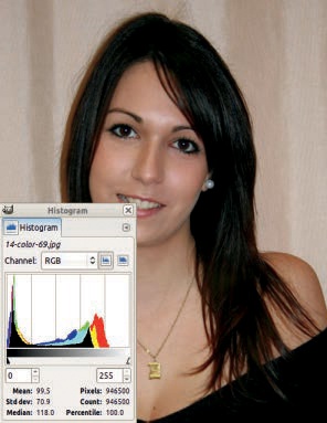
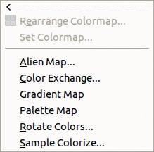
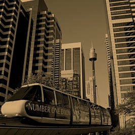
The Map submenu, shown in Figure 12-101, is separated into two sections. Tools in the first section apply only to images in Indexed mode. Tools in the second section apply only to images in RGB mode or, for some of the entries, Grayscale mode. We’ll use the image in Figure 12-102 as an example and convert a copy of it to Indexed mode with an optimal palette of 256 colors and Floyd-Steinberg dithering to demonstrate the first two tools (see Indexed Mode for more information about indexing).

This tool does not change the image. It simply changes the numbering of the entries in the colormap. As shown in Figure 12-103 (only a quarter of the actual window is visible), we can move the entries by dragging and dropping. Right-click anywhere in the window to sort the colormap according to one of the HSV components or to reverse or reset the order.
The Set Colormap tool opens a dialog in which we can only choose a new colormap from among those available (Figure 12-104). Some of the colormaps yield odd results, as you can see in Figure 12-105.
The Alien Map tool transforms the colors of an image in the RGB or the HSL model by applying trigonometric functions to the pixel values.
The dialog shown in Figure 12-106 begins with a preview. Then we choose the color model, called mode in this dialog. The checkboxes on the right control which of the channels will be affected.

Each channel has two sliders: frequency [0 to 20] and phaseshift [0 to 360]. Frequencies that are less than 0.7 yield a result similar to the original. Higher values give an increasingly “alien” result. Figure 12-107 is the result of using a frequency of 6.00 in the three RGB channels and a phaseshift of 0.00 in the three HSV channels.

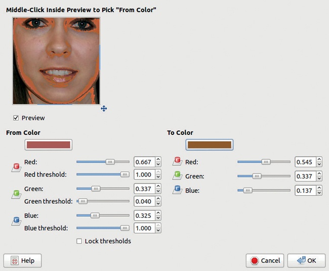
As its name indicates, this tool replaces a color in the image with a different one.
The dialog, shown in Figure 12-108, contains a preview that you middle-click to define the FROM COLOR. This color can also be defined by clicking the corresponding button, which opens the Color chooser, or by setting the three sliders for the RGB channels. Each channel also has threshold sliders [0 to 1], which you adjust to set how much of the channel will be replaced.
The pixels in the image that are similar to the chosen FROM COLOR, within the threshold limits, are replaced with the TO COLOR, which you select using the button or the three sliders.
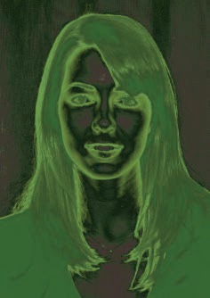
The Gradient Map tool has no dialog. It uses the current gradient, which you can change in the Gradients dialog, usually a dockable dialog in the multi-dialog window below the layers tab. The mapping occurs between the color intensities in the image (represented as the Value channel in the Levels tool, for example) and the colors in the gradient. The left end of the gradient is mapped to the darkest pixel, and the right end to the lightest pixel. Figure 12-109 shows the result using the Greens gradient.
The Palette Map tool works like the Gradient Map tool, only it uses the current palette instead of the current gradient. Change the current palette via the Palettes dialog. This dialog can be opened by clicking the small button to the right of any dockable dialog or from the Image: Windows > Dockable Dialogs menu. Figure 12-110 shows the result using the Gold palette.


The Rotate Colors tool uses the Hue color circle to alter the image colors. A hue subrange is defined on the FROM circle as a sector, and another sector is defined on the TO circle. The colors in the input range are mapped to the colors in the output range. The other colors are not affected.
This dialog is shown in Figure 12-111. You can adjust the two color ranges in various ways. The previews on the left show the original image and the current result. To get the dramatic change shown in Figure 12-112, we clicked the CHANGE ORDER OF ARROWS button.

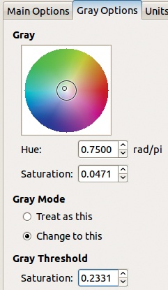
This dialog contains a second tab, shown in Figure 12-113. On this tab, we specify a color in the image to replace with gray, as long as the CHANGE TO THIS radio button is checked. The center circle is a visual representation of the GRAY THRESHOLD saturation: It extends when the threshold saturation is increased. The position of the small circle defines the hue and saturation of the color that will be converted to gray. If the TREAT AS THIS radio button is checked, the hue that will be converted to gray is defined by the rotation specified on the Main Options tab.
The Sample Colorize tool uses a sampling image to colorize a destination image.
The destination image must be in RGB mode but can be either grayscale or color. Its colors will be discarded; only the Value channel will be used in the resulting image. Figure 12-114 shows the dialog for this tool. We created a sample image by applying a linear gradient to a blank canvas, using the Blend tool and the Incandescent gradient. The drop-down menus at the top of the dialog contain all of the images currently open in GIMP; use them to select a sample or use the current gradient as the sample, either as is or reversed. We can use the triangles or the numbers below the sample image preview to restrict the output range. We can also change the prominence of dark, medium, and light tones, using the triangles or the numbers in the input range below the destination image preview.
Various checkboxes set the parameters. HOLD INTENSITY applies the average light intensity of the source image to the destination image. ORIGINAL INTENSITY inactivates the Input levels intensity settings. USE SUBCOLORS makes the colors of an output pixel a mixture of the source and destination image values; otherwise, only the dominant color (the color with the maximum value) is used. SMOOTH SAMPLES improves the transition between colors selected after clicking the GET SAMPLE COLORS button.
The Info submenu is shown in Figure 12-115. These entries don’t change the image. Rather, they offer ways to gather information about the image properties, which allow you to make informed adjustments using the other tools.


The Histogram tool opens a dockable dialog that can be selected via Image: Windows > Dockable Dialogs > Histogram and docked in one of the multi-dialog windows.
Keeping this dialog open on the screen is helpful, because it’s automatically updated when the current image changes and it provides a way to track the effect of various adjustments. Adjust its size, either to reduce the histogram and save space on the screen or to extend the histogram and show more precise information. In Figure 12-116, only the Value channel is displayed in linear mode. Numeric data about the image pixels is displayed at the bottom of the dialog: the mean, standard deviation, and median of the values, and the number of pixels.

In Figure 12-117, we’ve displayed the Red channel and defined a subrange by moving the white triangle below the histogram. Because this is an informational dialog, the image doesn’t change, but the data does: The pixel count is different from the total, and the percentile is less than 100.
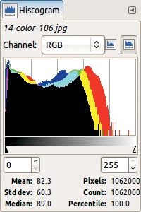
In Figure 12-118, we’ve displayed the three RGB channels at the same time, and the histogram is logarithmic. In Logarithmic mode, the low values are more prominent, which is generally better since small differences in small values are much easier to see than small differences in high values.

The Border Average tool is useful for finding an appropriate background color to go behind an image on a web page. It determines which color occurs most often along the border of the current layer and sets it as the foreground color. Because this does not change the image itself, this tool has no undo capability.
The Border Average dialog, shown in Figure 12-119, contains only two settings. The thickness of the BORDER SIZE specifies how much of the current layer is used in the calculation. The NUMBER OF COLORS is specified by the bucket size in the following way: Colors found in the border are placed in different buckets, depending on their similarity. The bucket containing the most colors is used to set the foreground color. A small bucket size leads to a large number of buckets and, often, an unexpected result. For example, when we applied the tool for the image in Figure 12-102, a bucket size of 16 yielded black, because the model’s black shirt spans much of the bottom border of the image and the tone is fairly consistent. A bucket size of 64 yielded a gray color, which is a mixture of the beige in the background of the photograph and the black of the woman’s shirt.
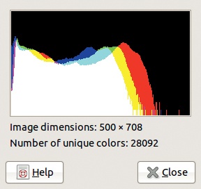
This tool has been more or less obsolete since GIMP 2.4: Its dialog (Figure 12-120) only displays the RGB logarithmic histogram, the image dimensions, and the number of unique colors.


This tool uses the various colors in the current layer to generate a palette in the form of a series of color stripes, as shown in Figure 12-121. We use it mainly with the Flame filter (see Flame).
In the dialog shown in Figure 12-122, the first two parameters set the dimensions of the new image for the palette. SEARCH DEPTH [1 to 1024] generates more colors when you increase the value.
The last part of the Colors menu contains six tools that aren’t really related but are grouped here. We’ll use the sample image shown in Figure 12-123 to demonstrate the effect of each of these tools.


The Color to Alpha tool replaces some chosen color with transparency. Its dialog, shown in Figure 12-124, contains a preview and a button for choosing the color, which opens a simplified version of the Color chooser. We chose a color from the picture using the eyedropper, and the result appears in Figure 12-125.
The Colorify tool desaturates the image and then colorizes it, as if it were a grayscale image seen through colored glass. The Colorify tool actually does the same thing as the Colorize tool but with a different user interface. Its dialog, shown in Figure 12-126, contains a preview; a small palette of fully saturated colors; and a button for defining a custom color, which opens a simplified version of the Color chooser. Choosing a light color is best because darker colors reduce the contrast in the image, as demonstrated in Figure 12-127.


As its name suggests, this entry is actually a collection of tools, called filters, although they don’t have any specific connection to the collection of tools found in the Image: Filters menu.

Its dialog, shown in Figure 12-128, contains the following options:
Two previews, before and after the filter. These previews are very small and you can’t zoom in, so we often find it useful to first make a small selection in the image, work on that selection, invert it, and apply the tool again with the same parameters.
SHOW allows you to change what’s shown in the preview. To use the trick just described, choose to show only the selection rather than the entire image.
The four checkboxes in WINDOWS open corresponding windows, which are explained next.
AFFECTED RANGE works in the same way as in the Color Balance tool (see Color Balance).
SELECT PIXELS BY further determines which subrange will be affected by the changes.
The ROUGHNESS slider [0 to 1] sets the strength of changes made when you click a window.

The windows, which open when the corresponding boxes in the Filter Pack dialog are checked, each contain a filter linked to the main dialog but offering a unique way to edit the image. The four windows are these:
HUE: Its dialog, shown in Figure 12-129, contains seven previews. The center one displays the current state of the image. The others correspond to the three RGB colors and their complementary colors. Clicking one of the previews adds the corresponding color to the selected subrange (set in the Filter Pack dialog) with the current ROUGHNESS. Subtract a color by clicking its complementary color.
SATURATION: Its dialog, shown in Figure 12-130, contains only three previews, allowing you to increase or decrease the saturation in the current subrange.
VALUE: Its dialog, shown in Figure 12-131, also contains three previews, allowing you to increase or decrease the value in the image.
ADVANCED: This checkbox opens the dialog shown in Figure 12-132. The PREVIEW SIZE slider [50 to 125] allows you to change the size of the preview slightly. The AFFECTED RANGE specifies the meaning of Shadows, Midtones, and Highlights. The blue triangle allows you to remove the darkest pixels from the affected subrange. You can use the two other triangles to define the limits of the three subranges. The shape of the curve depends on the range chosen in the main window, on the roughness, and on the position of the bottom slider [0 to 1]. This shape represents the intensity of the changes that will be made to the image.


The Hot tool selects pixels that could cause problems when displayed in NTSC or PAL video. In its dialog, shown in Figure 12-133, you can select the video mode as well as the process used to mitigate the potential problem. You can reduce luminance or saturation or blacken the pixels. By default, the changes made with this tool are done on an additional, transparent layer.
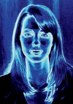
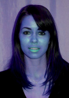
The Maximum RGB tool keeps only the RGB component with the maximum (or minimum) value. This explains why in its dialog, shown in Figure 12-134, the preview shows an image that’s mainly red, except for the eyes, which are blue. If we choose the minimal channels, the result is mainly blue, except for the eyes, which are now red.
Retinex algorithms are designed to mimic the dynamics of human vision, making images viewed on a screen appear more realistic. The human eye distinguishes colors even in poor or colored lighting. The Retinex tool uses the MSRCR algorithm, which is used in digital photography or for processing astronomical and medical photographs.

The options in its Figure 12-135, assume that the user has some knowledge of the mathematics of the Retinex MSRCR algorithm. Those who don’t possess the required knowledge can simply fiddle with the options and sliders until the result is appealing. An example is shown in Figure 12-136.

