
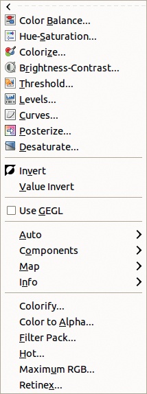
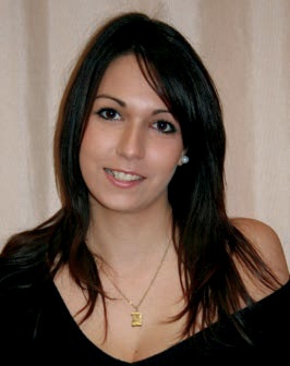
The Image: Colors menu contains lots of entries (see Figure 12-67). The first section of the menu contains the more basic tools, including Levels and Curves, which we just discussed. Now, we’ll demonstrate the other tools in this part of the menu using the photograph shown in Figure 12-68. (Tip: You can access these entries by placing them in the Toolbox or via Image: Tools > Color Tools.)
The adjustments you can make with the Color Balance tool can also be made with the Levels or Curves tool, but some people find the Color Balance tool more intuitive. Its dialog is shown in Figure 12-69. The top of this dialog contains the same settings as the Levels and Curves tools, settings that are also shared by the next four tools in the menu: Hue-Saturation, Colorize, Brightness-Contrast, and Threshold.
Adjust the color balance using three sliders [–100 to +100], one for each combination of a fundamental color and complementary color in the RGB and CMY models. Recall that the pairings are the same in these two models, but the designation of fundamental versus complementary differs.
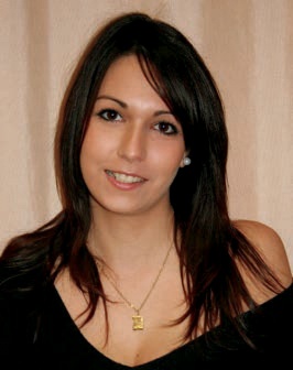
Balance tool to make adjustments in three different ranges: Shadows, Midtones, and Highlights. These ranges overlap, and precisely distinguishing them in an image is difficult. Because the sliders are very sensitive, achieving a natural-looking result is hard, as demonstrated in Figure 12-70. Each of the ranges can be reset individually (by setting the value to 0), which makes adjusting an image by trial and error easier. Leave the two boxes at the bottom of the dialog checked to preview the effects of an adjustment.

This tool offers yet another way to make adjustments that you could also make using the Curves tool. The advantage of Hue-Saturation is that the controls are based on the three color models: RGB, CMY, and HSV. Another important difference is that Hue-Saturation deals with color ranges rather than color channels. For example, how would you change the saturation of yellow pixels using the Curves tool? With Hue-Saturation, it’s easy.
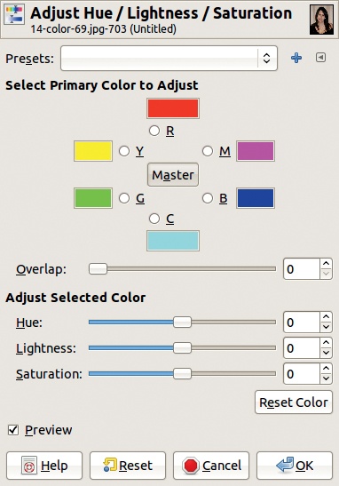
The Hue-Saturation dialog, shown in Figure 12-71, begins with the customary line for the PRESETS settings.

The next part of the dialog lets us select what color range to change. The center button, called MASTER, allows us to change all the colors simultaneously. The six colored buttons specify color ranges, each representing a sixth of the hue circle. The OVERLAP slider [0 to 100] extends the chosen range into the two neighboring ranges.
The next three sliders are based on the HSV model. (Here, Value is called Lightness). The effect of adjusting any of the three sliders is visible not only in the image but also in the color buttons in the upper part of the dialog. Adjust the hue, saturation, or lightness of any of the six colors, or select the Master control. The many different possible combinations make this tool a difficult one to master. One possible result of the Hue-Saturation tool is shown in Figure 12-72.
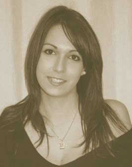

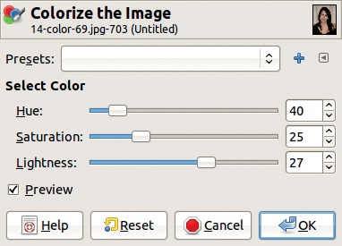
The Colorize tool first desaturates the image and then adds color to a grayscale version in RGB mode. Its dialog (Figure 12-73) begins with the standard color tool PRESETS option. Below that are sliders to specify the HSV components to apply to the image. The effect is similar to looking at a grayscale image through colored glass. The parameters shown in Figure 12-73 produce the sepia photograph in Figure 12-74.
The Brightness-Contrast tool is very simple, as you can see from its dialog (Figure 12-75). As the name implies, you can use it to adjust two characteristics of an image: brightness and contrast.

Because this tool’s abilities are rather limited, a button is included (EDIT THESE SETTINGS AS LEVELS) that opens the Levels tool, which you can use to edit brightness and contrast with much more flexibility. The sliders in the Brightness-Contrast tool work in the usual way, but when the tool is active, we can also click and drag in the image itself: Vertical strokes change the brightness, horizontal strokes change the contrast. Figure 12-76 shows the result of the settings shown in Figure 12-75.
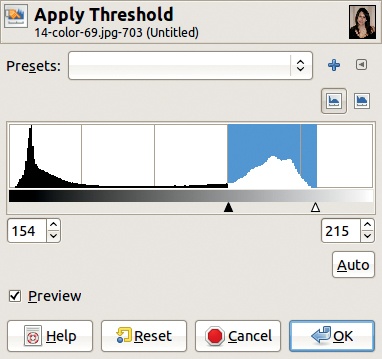
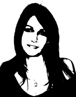
The Threshold tool transforms the current layer into a black and white image. Pixels that have a value within the set range are white, and those that have a value outside the range are black. Set the range by moving the two triangles below the histogram. Generally, you can achieve a better result by setting the threshold manually than by using the AUTO button. The settings shown in Figure 12-77 generate the result in Figure 12-78.
Use the Threshold tool to generate a natural mask, as described in Building a Natural Mask.
The Posterize tool reduces the number of colors in an image. The only slider, which has a range of [2 to 256], is used to set the number of colors in each RGB channel. Setting the level to 8 generates the result shown in Figure 12-79.
The Desaturate tool removes all color from the current layer, but the image remains in RGB mode, so you can add color later. The dialog includes three ways to compute the gray levels of the pixels.

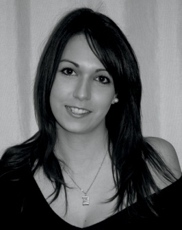
Figure 12-80 shows the result of applying LUMINOSITY.


The two inversion tools operate instantly on the current layer. Image: Colors > Invert generates the result shown in Figure 12-81. The colors are inverted (i.e., they are replaced by their complementary color, as in a photographic negative). Image: Colors > Value Invert generates the result shown in Figure 12-82. When this tool is used, only the Value component in the HSV model is inverted via the formula V = 100 – V, where V is the pixel value. Rounding errors can lead to a strong color distortion.

