
Almost everybody has a digital camera now and can take countless photographs without worrying about the cost of film or developing. Digital photographs are probably the most common type of images edited in GIMP. A wide range of digital cameras are on the market today, with prices ranging from less than ten dollars to tens of thousands of dollars. The CCD sensors generate from 1 megapixel to more than 50 megapixels for the most expensive models. The optics of a reflex camera account for a huge proportion of the total cost, with the many possible features and gadgets available contributing less to the cost.
Many, many models are on the market, and there are at least as many unique user needs, so we won’t offer any camera-shopping advice. If you need help choosing a camera, you can find detailed reviews online. From this point on, we assume you already have a camera in hand.
As you saw in the Image: File > Create menu, shown in Figure 19-1, two entries involve a camera, assuming the gtkam-gimp plug-in is installed. (If it is not, simply install the gtkam-gimp package as described in Appendix E.) CAPTURE FROM CAMERA allows you to take photographs from inside GIMP by controlling the camera. LOAD FROM CAMERA allows you to access the photographs stored on a camera’s memory card.
You don’t need to use GIMP to retrieve photographs from a camera, as several applications will do this. However, if you plan to edit your photographs in GIMP, retrieving them in GIMP can be simpler than using a complicated application for managing photo albums.
Note that you don’t have to connect the camera to the computer if you have a card reader. When the camera’s card is inserted into a reader, the computer treats it like a new storage disk.


You should see a hierarchy of folders with all the photographs as files in one or several folders. The files are named using a pattern specific to the camera. You can open one of these files in GIMP in the same way that you would open any saved file.
LOAD FROM CAMERA is useful when you want to load just one photograph from the camera, not a lot of photographs at once. When you select LOAD FROM CAMERA, you get the dialog shown in Figure 19-24. The name of the camera obviously depends on what model you have.
After choosing your camera and navigating through its folder hierarchy in the left frame of the dialog, you’ll arrive at the window shown in Figure 19-25, where thumbnails of the available photographs appear in the right frame. Now you can select one thumbnail and click OK to load the corresponding photograph into GIMP. The dialog then closes, and you’ll have to select it again if you want to load another photograph.
The simplest cameras store photographs in JPEG format only, due to the compression capabilities of this format. For example, if the camera’s CCD sensors generate 10 megapixels, then, assuming 3 bytes per pixel, a full photograph would take up 30MB. Even with a memory card of considerable size, this severely limits the number of pictures that you can store. Moreover, saving large image files onto the card takes time, so you wouldn’t be able to take several pictures in quick succession.
A high-quality camera should offer a choice among several definitions and several compression factors. Usually image files can range from 30KB for the lowest definition and highest compression factor to 4MB for the highest definition and lowest compression. Of course, the number of images the memory card can store is inversely related to the picture file size. Unless you want to take a lot of pictures in a short time, choose the best photograph quality: The result that you can get when editing a picture in GIMP is limited by the quality of the initial image. Although JPEG is standard, some people prefer TIFF because they say it uses a lossless compression algorithm. TIFF doesn’t actually use any compression algorithm, but a TIFF image may specify an algorithm, which can be lossless. It can also use a JPEG compression algorithm, which is lossy. A TIFF file is always much larger than the equivalent JPEG file and can’t be read by as many software applications. The TIFF format is actually a container for several formats, so there’s no guarantee that all the features specified in an image will be properly handled by an application. JPEG is a better choice for most users, and if a lossless format is absolutely needed, PNG is a better choice than TIFF.
The compression algorithm used by JPEG sometimes generates artifacts. If the quality factor is large enough, these artifacts won’t be visible, even when the image is zoomed in substantially. But you should avoid repeatedly exporting an image in the JPEG format because the compression deterioration is cumulative. Also, note that setting the quality factor higher than when the image was loaded is pointless. Doing so only increases the file size without actually increasing the quality.

Most quality cameras also allow you to save photographs in raw format, which is not a specific format. As many different raw formats exist as camera manufacturers, and the same manufacturer often defines different raw formats for different camera models. Moreover, all these raw formats are incompatible with each other, so the proprietary software used for decoding one is incompatible with the software released with a new camera model from the same manufacturer.
The main drawback of any raw format is that you have no guarantee you’ll be able to open files in a specific raw format in a few years. Raw format is, therefore, not a good choice for storing photographs. Choose an internationally standardized format; for photographs, JPEG with a high quality rate (85 or greater) is the best solution.
Raw format is often called the digital negative, but this term is misleading because raw format is a mathematical approximation of the image, whereas a true negative is the actual image projected on the back of the camera. The definition of a negative depends on the size of the crystals that compose it, but it’s always many times better than the definition of the best CCD matrix.
The reason the raw format is called a digital negative is that it represents the data emitted by the CCD sensors. These data are generally sampled to create 4096 different values, which equate to 12 bits per sensor. The sensors are arranged in a Bayer pattern, shown in Figure 19-26. Note that there are twice as many green cells as there are red and blue ones. This is because the human eye is much more sensitive to the green wavelengths.

Color pixels are interpolated from the information generated by the cells via Bayer interpolation, which is the first transformation done to the data. After that, the camera executes several successive processes: White balance, contrast, and saturation are adjusted, and the sharpness is enhanced, among other things.
Finally, the data generated are compressed to 8 bit and then compressed to JPEG format. The compression from 12 to 8 bit doesn’t cause much loss because the compression is logarithmic, which preserves information with precision where it is most needed: in the low values. But in the high values, only a few different brightness levels are retained. The information lost during the compression to JPEG can vary from nominal (with a high quality setting) to severe.
The one advantage of raw format is that it is the only format that allows you to do all the transformations to your images manually. People often promote the use of raw format because it allows for correcting extreme exposure errors. This assumption is partly true because less data are present after the automatic transformations. But if you know how to use your camera correctly, you probably won’t make mistakes that are too extreme for the camera to handle.
If you don’t mind complicated software applications and fiddling with numerous parameters, and you want full control over what happens after the sensors measure the light arriving on them, raw format might be for you. Also, if you absolutely need 16-bit depth and if you have a lot of time to spend on every photograph, then raw format is a fine choice. But as long as a high quality setting is used, JPEG isn’t inferior to raw format, although some people who present themselves as professionals might argue otherwise. Even if raw format is ideal for you, we recommend generating both raw and JPEG images, as long as you don’t need to take a lot of photographs very quickly. And you should always choose a different format (such as JPEG or XCF) for long-term storage.
If you do choose to work with raw images, you can use the generic, free software tool called UFRaw (see http://ufraw.sourceforge.net/), which reads most raw formats, is regularly updated, costs nothing, and is available on all GNU/Linux distributions, as well as on Mac OS X and various versions of Windows. You can use it as a separate application or as a GIMP plug-in.
Darktable (see http://www.darktable.org/) is a more powerful tool, also generic and free software. But it is not available for any version of Windows, and it’s not interfaced with GIMP. Thus, in this section we suppose that you installed UFRaw and the corresponding GIMP plug-in.
When you open a raw image in GIMP, it automatically calls the UFRaw plug-in, which displays the dialog shown in Figure 19-27. On the right is a preview of the image, with buttons for zooming in or out. On the left, you’ll see a number of information windows, tabs, buttons, sliders, and other controls. These controls show the transformation process that UFRaw applies to the image in place of the transformations normally done by the camera.
The top histogram shows the raw data coming from the sensor cells and the curves that represent how the data will be converted. The histogram is bunched up on the left, which means that most of the pixels have a low luminosity. By right-clicking the histogram, you can switch between a logarithmic view, as shown in Figure 19-28, and a linear view. In the same figure, we see the RGB values for whatever point we’ve clicked in the image, as well as the luminosity and the Adams zone.[1]


The row just below the raw histogram contains a slider for adjusting the exposure, two buttons for restoring highlights and controlling how corrections are applied, and a button for automatically adjusting the exposure.
Next are eight tabs, which you can use to set successive transformations that will be applied to the data:
White balance (Figure 19-29, top): The initial value is chosen on the camera but not applied to the raw data. The TEMPERATURE slider changes the relative amounts of warm and cool colors. The slider below is for adjusting the Green channel, which is not affected by the color temperature. Several preset white balance settings are available.
Interpolation (Figure 19-29, middle): This allows you to choose among several different algorithms for Bayer interpolation.
Grayscale (Figure 19-30): This tab contains a number of methods for generating a grayscale image from a color one.
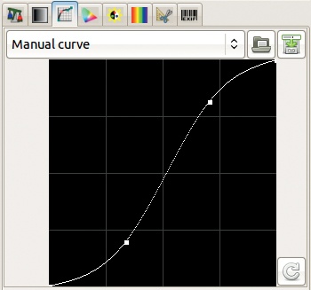
Base curve (Figure 19-31): This tab works like the Image: Colors > Curves tool, but it operates only on the Value channel.
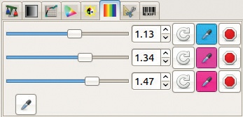
Color management (Figure 19-32): This tab contains settings for the various color parameters and for ICC profiles.
Saturation (Figure 19-33): This tab has a correction curve that works like the one for the Value channel.
Lightness adjustments (Figure 19-34): This tab lets you select up to three colors from the image and then to adjust its lightness from [0 to 2].
Lightness adjustments (Figure 19-34): This tab lets you select up to three colors from the image and then adjust its lightness in [0 to 2].
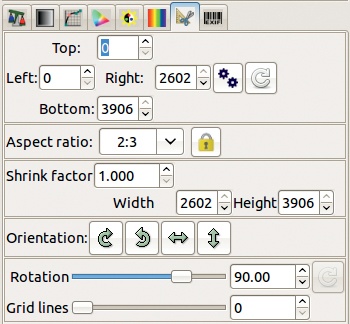
Crop and rotate (Figure 19-35): This tab contains some simple controls for cropping and rotating the image, but GIMP offers more powerful and convenient tools.
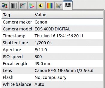
EXIF data (Figure 19-36): This tab lists information generated by the camera and describes how the picture was taken. This information cannot be changed.


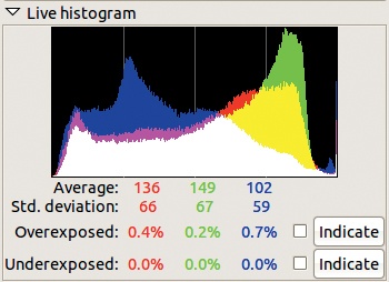
The final histogram (Figure 19-37) displays the properties the image will have when all the selected transformations are applied. You can select different display options by right-clicking. Various checkboxes and buttons reveal any of the overexposed or underexposed areas.
When you click OK, the transformations are applied to the image, and it’s loaded into GIMP.
[1] Ansel Adams is a celebrated photographer who defined the zone system to mitigate the exposure issues caused by the fact that light meters assume that the average of all scenes is middle gray. See http://www.normankoren.com/zonesystem.html for a more thorough explanation.