In this exercise, you’ll look at different views of an Excel workbook and experiment with ways you can move around in workbooks and worksheets. You’ll create a second instance of a workbook and open another workbook; then you’ll have Excel arrange the open windows in various ways. You can use many of the techniques you’ll practice in this exercise in other Office 2008 programs.
Note
SET UP This exercise uses the InvestmentCalculator and Loan workbooks located in the ~/Documents/Microsoft Press/2008OfficeMacSBS/OfficePrograms/ folder. Start Excel, and then follow the steps below.
Open the InvestmentCalculator workbook.
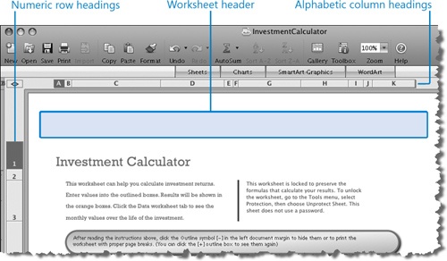
The workbook opens in Page Layout view.
If the entire page width isn’t visible as shown in the preceding graphic, click the green Restore button on the left end of the window header and then, in the Zoom list, click 100%.
This workbook includes two worksheets: Investment Calculator and Data. The worksheet header information is visible at the top of the worksheet, above Row 1.
The information on this worksheet occupies a total of 16 pages: 2 pages across and 8 pages down.
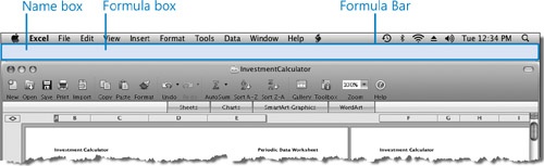
On the View menu, click Formula Bar.
The Formula Bar opens below the Excel menu bar. Notice that the Formula Bar, unlike most toolbars, is not integrated into the workbook window. It remains visible when Excel is active, regardless of whether a workbook is open.
Press Command+End to move to the last occupied cell on the worksheet.
Tip
By pressing Command+End, you can locate content that’s outside of your intended worksheet layout.
The cell reference (F364) appears in the Name box on the Formula Bar, and the formula calculating the cell value ($325,235.79) appears in the formula box.
Drag the vertical scroll box to the bottom of the scroll bar.
The worksheet content in the window moves so that only the last row is visible.
Click the Scroll Up button on the vertical scroll bar three times.
Rows 361 through 364 (displaying periods 357 through 361) are visible.
Click one time at the end of the content in the formula box.
The formula appears in cell F364 in place of its results. Cell references in the formula, and the corresponding cells in the worksheet, are identified by color.
Click anywhere in the formula.
A ScreenTip displays the correct formula syntax.
See Also
For information about Excel formulas, see Chapter 9.
Press the Escape key to deactivate the Formula Bar without making changes. Then click the red Close button at the left end of the Formula Bar to close it.
On the View toolbar in the lower-left corner of the workbook window, click the Normal View button.
The page layout representations, such as the headers and page margins, disappear.
Press the Home key to move to cell A364, at the beginning of the active row.
Press the Page Up key twice to move up two screens.
Press Control+Page Up to move to the Investment Calculator worksheet.
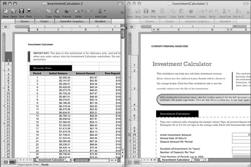
On the Window menu, click New Window.
Excel opens a second instance of the InvestmentCalculator workbook and appends numbers to the workbook names in the window title bars.
Drag the InvestmentCalculator:2 window down, by its title bar, so both windows are visible.
In the InvestmentCalculator:2 window, click the Data worksheet tab.
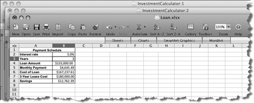
On the File menu, point to Open Recent, and then in the list, click Loan.xlsx.
Troubleshooting
If the Loan workbook doesn’t appear in the Open Recent list, open it from the ~/Documents/Microsoft Press/2008OfficeMacSBS/OfficePrograms/ folder.
You now have three open Excel workbook windows, containing different content, arranged in layers.
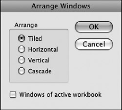
On the Window menu, click Arrange.
The Arrange Windows dialog box opens, depicting the most recent arrangement selection. If you haven’t previously arranged windows, the Tiled arrangement is selected.
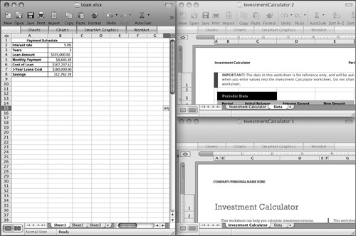
In the Arrange area, click Tiled. Then click OK.
Excel arranges the workbook windows so that all three are visible. In a tiled layout with an odd number of windows, the workbook that is active at the time of the arrangement (in this case, the Loan workbook) occupies the largest window.
Open the Arrange dialog box, click Cascade, and then click OK.
Excel stacks the three windows in neat layers, with the title bar of each window visible.
Press Control+Tab to cycle through the open windows. End with the InvestmentCalculator:2 window active.
Open the Arrange dialog box, click Vertical, and select the Windows of active workbook check box. Then click OK.
Excel arranges only the two InvestmentCalculator windows in vertical columns.
Close either of the InvestmentCalculator windows.
The window number disappears from the end of the workbook name in the title bar of the remaining window.