In this exercise, you’ll create a workbook from an existing worksheet, make a copy of the worksheet within the workbook, and rename the new worksheet. Then you’ll delete rows of data and selected cells, shifting and reformatting the remaining data so that it’s legible. Finally, you’ll insert a new worksheet and populate it with selections of data from other sheets.
Note
SET UP Open the AirQuality workbook from the ~/Documents/Microsoft Press/ 2008OfficeMacSBS/WorkSheets/ folder. This workbook consists of eight worksheets: one containing data for all of the United States and the others for specific regions.
In the lower-left corner of the workbook window, at the left end of the sheet tabs, click the Last Sheet button.
The sheet tabs shift within the tab area so that you can see the last sheet, Regions 7-10, and the Insert Sheet button.
Click the Region 5 sheet tab.
This sheet displays air quality information from the United States Environmental Protection Agency for locations in one region of the United States. This region, referred to as Region 5, includes the states of Illinois (IL), Indiana (IN), Michigan (MI), Minnesota (MN), Ohio (OH), and Wisconsin (WI).
Right-click the Region 5 sheet tab, and then click Move or Copy.
The Move Or Copy dialog box opens. The To Book box displays the name of the current workbook. The Before Sheet box includes all the visible sheets in the active workbook.
Click the To book list.
The list expands. It includes all the currently open workbooks and a (new book) option.
In the To book list, click (new book).
The Before Sheet box is now empty, because the new book doesn’t yet have sheets.
Select the Create a copy check box, and then click OK.
Excel creates a new workbook containing only the Region 5 sheet. The workbook opens in the default Page Layout view.
On the View menu, click Normal.
Later in this exercise, it will be simpler to work with the data in Normal view. By changing to Normal view now, all the copies you make of this worksheet will also be in Normal view.
Save the workbook in your ~/Documents/Microsoft Press/2008OfficeMacSBS/ WorkSheets/ folder as My Region 5.xlsx.
In the My Region 5 workbook, right-click the Region 5 sheet tab, and then click Move or Copy.
In the Move or Copy dialog box, click (move to end) in the Before Sheet box, select the Create a copy check box, and then click OK.
Excel creates a copy of the worksheet, named Region 5 (2).
Note
The Region 5 worksheet page orientation is landscape rather than portrait, because that is the orientation that was set for the Region 5 worksheet in the original workbook. The default orientation of a new worksheet is portrait. By copying the worksheet rather than copying data to a new worksheet, you retain the page layout, column widths, and row heights of the original page.
Right-click the Region 5 (2) sheet tab, and then click Rename.
With the current worksheet name selected, type Michigan, and then press Return.
Column P lists the state of each Metropolitan Statistical Area in Region 5. You will delete the data for Illinois (IL), Indiana (IN), Minnesota (MN), Ohio (OH), and Wisconsin (WI), leaving only the data for Michigan (MI).
On the Michigan worksheet, point to the row 2 heading. When the cursor changes to a solid right-pointing arrow, drag through the headings for rows 2 through 21 to select all the entries for the states of Illinois and Indiana.
Press the Delete key located on the keypad to the right of the Return key (not the Delete key in the upper-right corner of the alphanumeric keypad).
The data in rows 2 through 21 disappears, but the blank rows remain.
Press Command+Z to restore the deleted data. Then, with rows 2 through 21 still selected, click Delete on the Edit menu.
Excel deletes rows 2 through 21, moving the Michigan entries to the top of the data range.
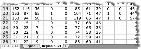
Click the row 10 heading. Then scroll the window if necessary, press and hold the Shift key, and click the row 34 heading.
Press the Delete key (again, the one on the keypad to the right of the Return key).
Excel deletes the Minnesota, Ohio, and Wisconsin entries, leaving only the eight Michigan entries. This method of deleting rows or columns of data works fine when no data follows the selected entries.
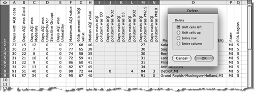
Drag to select cells I1 through N9. Then on the Edit menu, click Delete.
The Delete dialog box opens.
In the Delete dialog box, with Shift cells left selected, click OK.
Excel deletes the selected cells and shifts the remaining cells to the left to close the gap. Because we deleted cells rather than columns, the columns holding the shifted data aren’t the same width as their original columns.
Double-click the column separator between columns I and J to resize column I to fit its contents.
Select row 1, and then press Command+C to copy the column titles to the Clipboard.
At the right end of the sheet tabs, click the Insert Sheet button.
Excel creates a worksheet named Sheet3. The new worksheet is displayed in the default Page Layout view.
With cell A1 of the new worksheet active, press Command+V to paste the column titles into row 1 of Sheet3.
The titles appear at the top of the sheet, with the Paste Options button visible below cell A1.
Click the Paste Options button and then, in the list, click Keep Source Column Widths.
The columns in Sheet3 are resized to match those in the Michigan sheet.
Change the name of Sheet3 to Illinois.
Click the Region 5 sheet tab. Drag to select cells A2:H10 (A2 through H10). Then hold down the Command key and drag to select cells O2:Q10.
Press Command+C to copy the selected data to the Clipboard.
Click the Illinois sheet tab, click cell A2, and then press Command+V to paste the copied data into the Illinois sheet.
Notice that Excel pastes the data into the Illinois sheet without including the gap for the cells you didn’t select from the Region 5 sheet. Pretty slick!