In this exercise, you’ll first create a blank workbook. You’ll enter information into a worksheet and resize columns so that you can see the information. Then you’ll create additional data by copying and filling data series.
Note
SET UP This one’s easy—we’ll just jump right in! No practice files are required for this exercise.
Start Excel. (If Excel is already started, you’re a step ahead of the game.)
As with Word, starting the program (without opening a specific workbook) creates a blank temporary file—in Excel, this is a workbook named Workbook1.
On the toolbar, click the New button.
A blank workbook opens in Page Layout view, which is the default view for new workbooks. The upper-left cell, cell A1, is active. This is indicated by the blue outline of cell A1 and the shading of the column A heading and the row 1 heading.
With cell A1 active, type Item.
As you type, the text entry box for the cell you’re typing in pops up from the surrounding worksheet. This nifty little feature, which you won’t find in Excel 2007 for Windows, makes it much easier to distinguish the content of the active cell from that of the surrounding cells. Most conveniently, though, the pop-up displays all the text in the cell, so if there is more text than can be displayed in the cell, you can see it all while you’re editing it.
While you’re entering text, a blinking insertion point appears in the cell.
Press the Tab key.
Cell B1 becomes active. Notice that now there is no visible insertion point in the active cell.
In cell B1, type Room. Press Tab to move to cell C1, and type Description. Press
Tab to move to cell D1, and type Purchase Date.
As you type the final letter of the word Date, the text exceeds the width of the cell, and the text entry box expands to two columns wide.
Press Tab to move to cell E1, and type Purchase Price. Then press Return.
Pressing Return indicates to Excel that you’ve reached the end of the information you’re entering in this row. The cell selector moves to the cell that Excel perceives as the first in the series of data you’re entering. In this case, that should be cell A2. If you stopped to experiment with anything between steps 4 and 6, it might be cell B2 or C2.
Type the following data into cells A2 through E2:
In cell...
Type...
A2
1
B2
Dining Room
C2
Dining set (table and 8 chairs)
D2
2007
E2
2600
When you finish, press Return.
Some of the data isn’t visible because it’s larger than the cell it’s in, so let’s adjust the column width.
Note
The default worksheet font is 10-point Verdana. You can change the default font from the General page of the Excel Preferences dialog box. For example, you might want to use a larger font that is easier to see, use a smaller font to fit more on a page, or consistently use a font that is part of your corporate branding scheme.
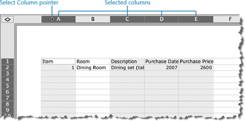
Point to the column C heading. When the pointer changes to a downward-pointing arrow, drag to the right through column E.
Hold down the Command key, and then click the column A heading.
Columns A, C, D, and E are now selected.
Point to the column separator to the right of column A. When the pointer changes to a double-headed horizontal arrow, double-click.
The width of each of the four selected columns changes to precisely fit its widest content.
Tip
If you have difficulty resizing the selected columns by double-clicking the column separator, you can instead point to Columns on the Format menu, and then click AutoFit Selection.
Later in this book we’ll apply character and paragraph formatting to the actual cell content.
Click cell A2, which contains the number 1.
Point to the fill handle in the lower-right corner of the active cell. When the pointer changes to a black plus sign, drag down through cell A11.
As you drag, the pointer changes to a diamond, with small arrows in the upper-left and lower-right corners, and a small box displays the value that will be entered in the cell.
When you release the mouse button, the number 1 appears in cells A2 through A11. The Auto Fill Options button appears outside the lower-right corner of the filled selection. If you don’t click this button, it will disappear on its own shortly.
Click the Auto Fill Options button to display a menu of options for filling the selected cells.
The Copy Cells option is currently selected. As a result, all the cells are filled with a replica of the initially selected cell.
On the Auto Fill Options menu, click Fill Series.
The contents of cells A2 through A11 change from a series of 1s to the numbers 1 through 10. The Auto Fill Options button remains available in case you want to choose a different option.
Tip
Auto Fill is one of the few actions that you can’t undo. If you Auto Fill a selection and don’t like the results, delete the filled data (but not the original base data) and start again.
We’ll do more with this worksheet later.
On the toolbar, click Save (or press Command+S).
The Save As dialog box opens. Notice that Excel suggests Workbook2 as the file name, rather than suggesting the first word in the file, as Word does.
In the Save As box, replace the suggested file name with My Inventory.
If the navigation area isn’t already visible in the Save As dialog box, click the Expand button to display it. Navigate to the ~/Documents/Microsoft Press/ 2008OfficeMacSBS/CreateWorkbooks/ folder.
In the Save As dialog box, click Save.
Excel saves the workbook, and the new file name appears on its title bar.