
Intersections: The Next Step Up
Ask yourself the following question: “Did I understand why we did what we did to build the cul-de-sac in the previous section?” If the answer is “Not really,” you may want to review a few topics before proceeding. If the answer is, “Yeah, mostly,” then you are ready to move to the next level of corridor complexity: intersections.
The steps that follow apply to all intersections, regardless of whether it is a T-shaped intersection, a four-way intersection, perfectly perpendicular, or skewed at an angle.
Corridor modeling is an iterative process. The more advanced your model, the more iterations it may take to get to the correct design. You will often not know the final design parameters until you see how the model relates to existing conditions or ties into other pieces of the design. Get comfortable jumping in and out of corridor properties and identifying regions within your corridor.
Plan what alignments, profiles, and assemblies you’ll need to create the right combination of baselines, regions, and targets to model an intersection that will interact the way you want. It helps to create a simple sketch, as shown in Figure 10-26.
Figure 10-26: Plan your intersection model in sketch form.

Figure 10-27 shows a sketch of required baselines. As you saw in the previous example, baselines are the horizontal and vertical foundation of a corridor. Each baseline consists of an alignment and its corresponding finished ground (FG) profile. You may never have thought of edge of pavement (EOP) in terms of profiles, but after building a few intersections, thinking that way will become second nature. The Intersection tool on the Create Design panel of the Home tab will create EOP baselines as curb return alignments for you, but it will rely on your input for curb return radii.
Figure 10-27: Required baselines for modeling a typical intersection
Figure 10-28 breaks each baseline into regions where a different assembly or different target will be applied. Once the intersection has been created, target mapping as well as other particulars can be modified as needed.
Figure 10-28: Required regions for modeling an intersection created by the Intersection tool

Using the Intersection Wizard
All the work of setting baselines, creating regions, setting targets, and applying the correct frequencies can be done manually for an intersection. However, Civil 3D contains an automated Intersection tool that can handle many types of intersections.
On the basis of the schematic you drew of your intersection, your main road will need several assemblies to reflect the different road cross sections. Figure 10-29 shows the full range of potential assemblies you may need in an intersection and the design situations in which they may arise.
Figure 10-29: Various assembly schematics and applications
Assembly Sets
When you are ready to create an intersection, you do not need to have all the special assemblies created. On the Corridor Regions page of the Create Intersection wizard, you will see a list of the assemblies Civil 3D plans to use. If the assemblies are not already part of the drawing, they will get pulled in automatically when you click Create Intersection.
The default intersection assemblies are general and may not work for your design situation. You will want to create and save an assembly set of your own.

In a file that contains all of your desired assemblies, work through the Create Intersection wizard to get to the Corridor Regions page. Click the ellipsis to select the appropriate assembly for each Corridor Region Section Type. Once the listing is complete, click the Save As A Set button.
Civil 3D creates an XML file that stores the listing of the assemblies. It also creates a copy of each assembly as a separate DWG file. Save the set in a network shared location so your office colleagues can use the set as well.
The next time an intersection is created, you can use the assembly set by clicking Browse and selecting the XML file. Civil 3D will pull in your assemblies, saving lots of time!
This exercise will take you through building a typical peer-road intersection using the Create Intersection wizard:
1. Open the Intersection.dwg file, which you can download from this book’s web page. The drawing contains two centerline alignments (USH 10 and Mill Creek Drive) that are part of the same corridor.
2. Select the corridor in plan view to activate the contextual tab. From the Modify Corridor panel, click Corridor Properties. Switch to the Parameters tab.
There are already two baselines with three regions each in the corridor. These are the regions for modeling the areas outside of the intersection. The regions that use the Null Assembly are empty placeholders to prevent feature lines from crossing through the intersection. This way, there is an empty spot for the corridor design to reside.
3. After making note of the current state of the corridor, click OK to close the Corridor Properties.
4. From the Home tab, choose the Intersections Create Intersection tool on the Create Design panel. Using the Intersection object snap, choose the intersection of the two existing alignments.
5. When prompted to select the main road alignment, click the USH 10 alignment that runs vertically in the project.
6. The Create Intersection – General dialog will appear (Figure 10-30). Name the intersection USH 10 and Mill Creek Drive. Set the Intersection corridor type to Primary Road Crown Maintained, as shown in Figure 10-30, and click Next.
Figure 10-30: The Create Intersection – General dialog

7. In the Geometry Details page (Figure 10-31), verify that USH 10 is the primary road by looking at the Priority listing. If USH 10 is not at the top of the list, use the arrow buttons on the right side.
Figure 10-31: The Geometry Details page of the Create Intersection wizard
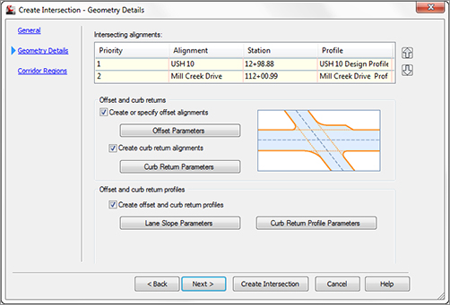
8. Click the Offset Parameters button.
- Set the offset values for both the left and right sides to 24′ for USH 10.
- Set the left and right offset values for Mill Creek Drive to 18′.
- Select the check box Create New Offsets From Start To End Of Centerlines.
- At this step, the screen should resemble Figure 10-32. Click OK to close the Offset Parameters dialog.
Figure 10-32: Intersection offset parameters

9. Click the Curb Return Parameters to enter the Curb Return Parameters dialog.
- For all four quadrants of the intersection, place a check mark next to Widen Turn Lane For Incoming Road and Widen Turn Lane For Outgoing Road.
- Click the Next button at the top of the dialog to move from quadrant to quadrant. As shown in Figure 10-33, a temporary glyph will help you determine which quadrant you are currently modifying.
Figure 10-33: Adding lane widening to the SW - Quadrant of the intersection

- For all four curb returns, click the check marks for Widen Turn Lane For Incoming Road and Widen Turn Lane For Outgoing Road. Leave turn lane values at their defaults for each quadrant.
- When you reach the last quadrant, you will see that the Next button is grayed out. This means that you have successfully worked through all four curb returns.
- Click OK to return to wizard’s Geometry Details page.
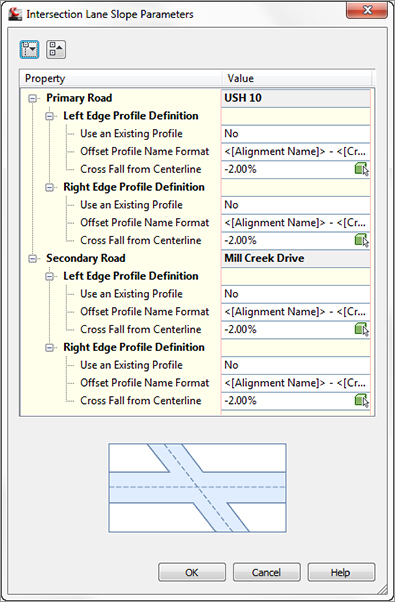
Some locales require that lane slopes flatten out to a 1 percent cross-slope in an intersection. If this is the case for you, you can change the lane slope parameters in the Intersection Lane Slope Parameters dialog (Figure 10-34).
Figure 10-34: Lane slope parameters control the cross-slope in the intersection.
Civil 3D is performing the task of generating the curb return profile. The profile will be at least as long as the rounded curb plus the turn lanes that are added in this exercise. If you wish to have Civil 3D generate even more than the length needed, you can specify that in the Intersection Curb Return Profile Parameters area (Figure 10-35).
Figure 10-35: Curb Return Profile Parameters extend the Civil 3D–generated profile beyond the curb returns by the value specified.

10. We will be keeping all default settings in both the Lane Slope Parameters area (Figure 10-34) and the Curb Return Parameters area (Figure 10-35). Click Next to continue to the Corridor Regions page (Figure 10-36).
Figure 10-36: The Corridor Regions page drives the assemblies used in the intersection.
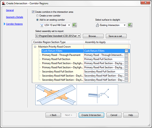
The Corridor Regions page is where you control which assemblies are used for the different design locations around the intersection. Clicking each entry in the Corridor Region Section Type list will give you a clear picture of which assemblies you should use and where (as shown at the bottom of Figure 10-36). If your assemblies have the same names as the default assemblies, as is the case in this example, they will be pulled from the current drawing. Alternately, you can click the ellipsis to select any assembly from the drawing.
If you don’t have all the necessary assemblies at this point, you can still create your intersection. Civil 3D will pull in the default set of assemblies. You can always modify these assemblies after they are brought in.
11. Set the Create Corridor In Intersection option to Add To An Existing Corridor. Click through the Corridor Region Section Type list to view the schematic preview for each. Do not make any changes to the assembly listing. Click Create Intersection.
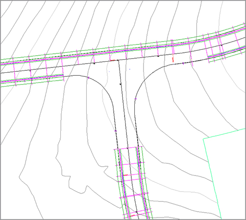
12. After a few moments of processing, you will see a corridor appear at the intersection of the roads. Use the REGEN command if you do not see the frequency lines. Your corridor should now resemble Figure 10-37.
Figure 10-37: The nearly completed intersection

Notice there are still some gaps where our initial corridor regions do not meet up with our corridor. In the next step, you will use grips to extend the regions to meet the intersection portion of the corridor.
13. Select the corridor. Use the diamond-shaped grips to pull the regions in toward the intersection, as shown in Figure 10-38a. If you are having difficulty doing so or are having computer performance problems, you can also adjust the region stations in the Parameters tab of the Corridor Properties dialog (Figure 10-38b).
Figure 10-38: Change the regions leading up to the intersections using grips (a) or in Corridor Properties (b)

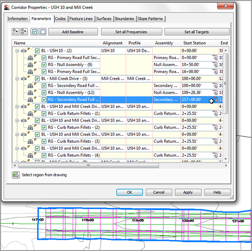
Notice how the region highlighted in the Parameters tab lights up graphically as well. This will help you determine which region to edit, even in the largest of corridors.
To move from region to region without searching through the somewhat daunting list, use the Select Region From Drawing button.
When the corridor is complete, it will look like Figure 10-39.
Figure 10-39: The completed intersection

Manually Modeling an Intersection
In some cases, you may find it necessary to model an intersection manually. Five-way intersections and intersections containing superelevated curves can’t be created with the automated tools alone. You need to understand what the intersection tool is doing behind the scenes before you can be a true corridor guru. The next example will take you through an overview of the manual steps.
At the point where the example begins, a few pieces are already in place: the centerline alignments and profiles, EOP alignments and profiles, and the full road assemblies. The corridor for the intersection is started for you, but it only contains one baseline. For simplicity's sake, daylight subassemblies have been omitted from this example.
In this example, you’ll add a baseline for an intersecting road to your corridor:
1. Open the Manual Intersection.dwg file, which you can download from this book’s web page.
2. Open the Corridor Properties dialog for Intersection1 (Cab-Syrah), and switch to the Parameters tab.
3. Click Add Baseline. The Pick Horizontal Alignment dialog opens.
4. Pick Syrah Way alignment. Click OK to dismiss the dialog.
5. Click in the Profile field on the Parameters tab of the Corridor Properties dialog. The Select A Profile dialog opens.
6. Pick the Syrah Way FG. Click OK to dismiss the dialog.
You now have a new baseline, but the region still needs to be added.
7. In the Corridors Properties dialog, right-click BL - Syrah Way and select Add Region.
8. In the Pick an Assembly dialog, select Full Road Section. Click OK to dismiss the dialog.
9. Expand BL - Syrah Way by clicking the small + sign, and see the new region you just created.
10. Click OK to dismiss the Corridor Properties dialog; your corridor will automatically rebuild. Your corridor should now look like Figure 10-40.
Figure 10-40: The Syrah Way baseline added

Notice that the region for the second baseline extends all the way through the intersection. You must now split the Syrah region to accommodate the curb returns.
11. Open the Corridor Properties dialog and switch to the Parameters tab. Using the techniques covered in the previous exercise, right-click to split the region at 3+50.00 and 5+50.00.
12. Switch the middle subassembly to Daylight Right. Your corridor parameters will now match Figure 10-41.
Figure 10-41: Split the Syrah Way baseline into 3 regions to accommodate curb returns

13. Click OK to update the corridor. You will see that the way has been cleared for the curb assemblies to be applied as shown in Figure 10-42.
Figure 10-42: The intersection corridor…so far
Creating an Assembly for the Intersection
You built several assemblies in Chapter 8, “Assemblies and Subassemblies,” but most of them were based on the paradigm of using the assembly marker along a centerline. This next exercise leads you through building an assembly that attaches at the EOP.
This exercise uses the LaneOutsideSuper subassembly (see Figure 10-43), but you’re by no means limited to this subassembly in practice.
Figure 10-43: An assembly for an intersection curb return
You can also use the LaneInsideSuper and LaneTowardCrown subassemblies, as well as any other lane with an alignment and profile target.
To create an assembly suitable for use on the filleted alignments of the intersection, follow these steps:
1. Open the Manual Intersection_Assembly.dwg file (which you can download from this book’s web page), or continue working in your drawing from the previous exercise.
2. From Prospector, expand the Assemblies group and locate Curb Return Fillets. Right-click on this assembly and select Zoom To. The assembly base has been placed in the drawing for you but does not contain any subassemblies.
3. Open your tool palette, and switch to the Lanes palette.
4. Click the LaneOutsideSuper subassembly. On the Properties palette, change the side to Left.
5. Click on the main baseline assembly to add the LaneOutsideSuper subassembly to the left side of the assembly.
6. Switch to the Curbs tab of the tool palette. Select UrbanCurbGutterGeneral. Change the side to Right and leave all other values at their defaults. Click to add the curb and gutter to the right side of the assembly.
7. Also on the Curbs tab of the tool palette, add an UrbanSidewalk assembly. Set the boulevard widths to 2′ for both inside and outside. Click to place the assembly.
You could combine steps 6 and 7 by using the Copy To Assembly option after selecting the curb and gutter along with the sidewalk from the Daylight Right Assembly.
Your assembly should now look like Figure 10-43.
Take the Pebble from My Hand, Grasshopper
If you are a little worried about the downward slope of the lane in the subassembly you just created, you needn’t be. Remember that the slope and length of the lane will be controlled by the alignment and profile target in the corridor. The geometry that you see in the assembly is purely preliminary. If this concept makes sense to you, you are ready for bigger and better corridors!
And of course, if you’d rather see that slope go +2% in the subassembly, you can change it in the good old AutoCAD properties, but keep in mind it won’t make one bit of difference to the corridor.
Adding Baselines, Regions, and Targets for the Intersections
The Intersection assembly attaches to alignments created along the EOP. Because a baseline requires both horizontal and vertical information, you also need to make sure that every EOP alignment has a corresponding finished ground (FG) profile.
It may seem awkward at first to create alignment and profiles for things like the EOP, but after some practice you’ll start to see things differently. If you’ve been designing intersections using 3D polylines or feature lines, think of the profile as a vertical representation of a feature line and the profile grid view as the feature-line elevation editor. If you’ve designed intersections by setting points, think of alignment PIs and profile PVIs as points. If you need a low point midway through the EOP, as indicated in the sketch at the beginning of this section, you’ll add a PVI with the appropriate elevation to the EOP FG profile.
Here are some things to keep in mind:
Site Geometry Make sure any alignments you create are either siteless (placed on the <none> site) or placed on another appropriate site.
Naming Conventions Instead of allowing your alignments and profiles to be named Alignment-1, Alignment-2, and so on, give each one a meaningful name that will help you keep them straight so that you can identify them on a list and locate them in plan. The same rule applies for the FG profiles. If the alignment is named EOP Right, then name the profile EOP Right FG or something similar. Explore alignment- and profile-name templates to see if you can help yourself by automating the naming.
Organization Figure out a way to keep your profile views organized. Perhaps line them up next to the appropriate road centerline, or use some other convention. If you just stick them anywhere, you’ll have a difficult time navigating and finding what you need.
Using Multiple Targets
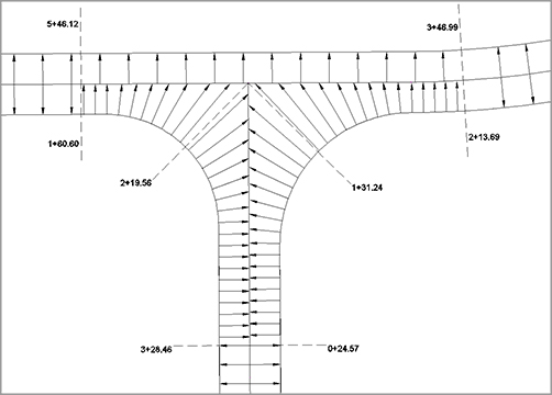
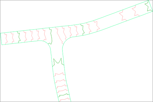
Civil 3D allows you to select more than one item in Width Or Offset Target and Slope Or Elevation Target areas. You can use any number of targets. You can even mix and match the types of targets you use, such as alignments with polylines, survey figures, and feature lines.
In the example that follows, you need two alignment targets and two profile targets in each curb region. To help Civil 3D figure out what you want, you need to verify that it will use the target that it finds first as it radiates out from the baseline. In most cases, you can click the Target To Nearest Offset option found in the target selection dialogs.

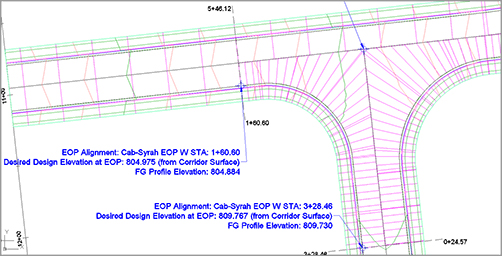
In the following graphic, the arrows represent the assemblies seeking out a target. From station 1+60.60 to 2+19.56, the Syrah Way alignment is closer to the baseline; therefore, Syrah Way’s geometry is used as the target. From station 2+19.56 to 3+28.46, Cabernet Court’s alignment is closer and is used as the target.
You’ll finalize the corridor intersection in the next exercise. Along the way, you’ll examine the corridor in various stages of completion so that you’ll understand what each step accomplishes. In practice, you’ll likely continue working until you build the entire model. Follow these steps:
1. Open the Manual Intersection_Targets.dwg file (which you can download from this book’s web page), or continue working in your drawing from the previous exercise.
2. (Optional) Zoom to the area where the profile views are located. Notice that existing and proposed ground profiles are created for both EOP alignments (see Figure 10-44). The step of developing the design profiles has been completed for you.
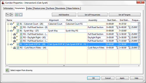
Figure 10-44: The Parameters tab with a new baseline and region
3. Select the corridor. Open the Corridor Properties dialog and switch to the Parameters tab.
4. Click Add Baseline. The Pick Horizontal Alignment dialog opens.
5. Select the Cab-Syrah EOP W alignment. Click OK to dismiss the dialog.
6. Click in the Profile field on the Parameters tab of the Corridor Properties dialog.
7. In the Select A Profile dialog, select Cab-Syrah EOP W- FG. Click OK to dismiss the dialog.
8. Right-click BL - Cab-Syrah EOP W and select Add Region.
9. In the Pick An Assembly dialog, select Curb Return Fillets. Click OK to dismiss the dialog.
10. Expand the baseline, and see the new region you just created. The Parameters tab of the Corridor Properties dialog will look like Figure 10-44.
11. Click OK to dismiss the Corridor Properties dialog and automatically rebuild your corridor. Your corridor should now look similar to Figure 10-45.
Figure 10-45: Your corridor after applying the Curb Return Fillets assembly
What is missing from the corridor? We need to rein in the station range, to set targets, and to add more frequency lines along the curves. Oh, and eventually we’ll want to do this all to the east side of the road as well.
12. Select the corridor in plan view, click Corridor Properties from the contextual tab, and switch to the Parameters tab. To set the correct stations for the regions, use the station picker and snap to where we stopped the main assembly along Syrah Way. This will be station 1+60.60. Set the end station using the station picker and snapping to where the normal region ends on Cabernet Court. This will be station 3+28.46.
13. Next, set the frequency by clicking the ellipsis button. Set both tangents and curves to 5′ . Click OK.
14. Click the ellipsis for targets.
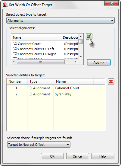
- Click the Width Alignment target for LaneOutsideSuper. Click the Select From Drawing button. Click both Syrah Way and Cabernet Court centerline alignments.
- Press ↵ when complete.
- In the Set Width Or Offset Target dialog, click Add. Both alignments will appear in the listing, as shown in Figure 10-46.
Figure 10-46: In the Set Width Or Offset Target dialog, use the Select From Drawing button to pick both Syrah Way and Cabernet Court centerlines.
- Click OK when complete.
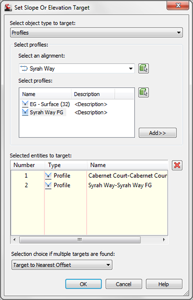
15. Click the Outside Elevation Profile target for LaneOutsideSuper.
- From the Select and Alignment drop-down, select Cabernet Court from the list.
- Highlight the Cabernet Court FG profile and click Add.
- Change the selected alignment to Syrah Way.
- Highlight the Syrah Way FG profile and again click Add. Both profiles will appear in the listing, as shown in Figure 10-47.
Figure 10-47: In the Set Slope Or Elevation Target dialog, pick alignment first, and then add the FG profile.
- Click OK.
16. Click OK to dismiss target mapping. Click OK to let the corridor build. Your intersection should now look like Figure 10-48.
Figure 10-48: Three baselines completed—one to go

17. Repeat steps 4–17 for the Cab-Syrah EOP E. Here are some hints to get you going: The region should go from station 0+24.57 to 2+13.69. The frequency should be 5′ for both tangents and curves. The target mapping will be identical to the region you created in steps 15–16.
18. Let the corridor build one last time and admire your work. The completed intersection should look like Figure 10-49.
Figure 10-49: The completed intersection

Troubleshooting Your Intersection
The best way to learn how to build advanced corridor components is to go ahead and build them, make mistakes, and try again. This section provides some guidelines on how to “read” your intersection to identify what steps you may have missed.
Your lanes appear to be backward. Occasionally, you may find that your lanes wind up on the wrong side of the EOP alignment, as in Figure 10-50. The most common cause is that your assembly is backwards from what is needed based on your alignment direction.
Figure 10-50: An intersection with the lanes modeled on the wrong side

Fix this problem by editing your subassembly to swap the lane to the other side of the assembly. If the assembly is used in another region that is correct, just make a new assembly that is the mirror reverse of the other assembly and apply the new one to the alignment.
In this exercise, you used an intersection assembly with the transition lane on the left side, so you made sure the left intersection EOP alignment ran clockwise and the right intersection EOP alignment ran counterclockwise. It’s also easy to reverse an alignment and quickly rebuild the corridor if you catch the mistake after the corridor is built.
Your intersection drops down to zero. A common problem when modeling corridors is the cliff effect, where a portion of your corridor drops down to zero. You probably won’t notice in plan view, but if you rotate your corridor in 3D using the Object Viewer (see Figure 10-51), you’ll see the problem. The most common cause for this phenomenon is incorrect region stationing.
Figure 10-51: A corridor viewed in 3D, showing a drop down to zero
Fix this problem by making sure your baseline profile exists where you need it and make note of the station range. Set your station range in the corridor to be within the correct range.
Your lanes extend too far in some directions. There are several variations on this problem, but they all appear similar to Figure 10-52. All or some of your lanes extend too far down a target alignment, or they may cross one another, and so on.
Figure 10-52: The intersection lanes extend too far down the main road alignment.

This occurs when a target alignment and profile have been omitted for one or more regions. In the case of Figure 10-52, the EOP Left baseline region was only set to one alignment. In an intersection, you need two targets in a corner region to model the road correctly.
Your lanes don’t extend far enough. If your intersection or portions of your intersection look like Figure 10-53, you neglected to set the correct target alignment and profile.
Figure 10-53: Intersection lanes don’t extend out far enough.

You can fix this problem by opening the Target Mapping dialog for the appropriate regions and double-checking that you assigned targets to the right subassembly. It’s also common to accidentally set the target for the wrong subassembly if you use Map All Targets or if you have poor naming conventions for your subassemblies.
Checking and Fine-Tuning the Corridor Model
Recall that the EOP profiles are developed by creating a preliminary corridor surface model. To create the EOP elevations, you filled in the gaps by creating the EOP design profile where the preliminary surface stops and picks back up again on the adjacent road (or in the case of the cul-de-sac, the opposite side of the street).
You will want to check the elevations of the corridor model against the profiles you created. The preliminary surface model was a best guess for elevations; now we need to reconcile our corridor geometry with those best-guess profiles. Figure 10-54 shows a common elevation problem that arises in the first iteration of intersection design.
Figure 10-54: A potential elevation problem in the intersection
The first step in correcting this is creating a corridor surface model out of Top links. The surface will show us exactly how Civil 3D is interpreting our design, elevation-wise.
Before beginning this exercise, review the basic corridor surface building sections in Chapter 9. When you think you are ready, follow these steps:
1. Open the Manual Intersection_Surface.dwg file (which you can download from this book’s web page), or continue working in your drawing from the previous exercise.
2. Select the corridor in plan view, click Corridor Properties from the contextual tab, and switch to the Surfaces tab.
3. Click the Create A Corridor Surface button. A Corridor Surface entry appears. Rename the surface to Corridor Surface by clicking on the surface name.
4. Ensure that Links is selected as Data Type and that Top appears under Specify Code. Click the + button. An entry for Top appears under the Corridor Surface entry.
5. Switch to the Boundaries tab. Right-click on Corridor Surface and select Corridor Extents as the outer boundary.
6. Click OK, and your corridor will automatically rebuild.
7. Freeze the corridor to get a better look at the corridor surface. You should have a corridor surface that appears similar to Figure 10-55.
Figure 10-55: A first-draft corridor surface
8. Thaw any frozen layers.
The next exercise will lead you through placing some design labels to assist in perfecting your model and then show you how to easily edit your EOP FG profiles to match the design intent on the basis of the draft corridor surface built in the previous section.
Don’t forget a few basics that will help you navigate this exercise easier. If you wish to see the drawing without the corridor, then freeze the corridor layer, which is C-ROAD-CORR-INTR. You can change the view of your surface around by changing the active style or by freezing C-TOPO. Also, remember that draw order may be an issue. You will have corridor feature lines overlapping alignments, so it may be best to use the Send To Back option on the corridor.
1. Open the Manual Intersection_Labels.dwg file (which you can download from this book’s web page), or continue working in your drawing from the previous exercise.
2. For the next few steps, either freeze the corridor layer or send your corridor display order to back.
3. Switch to the Annotate tab on the Ribbon. Click the Add Labels button. The Add Labels dialog box will appear.
4. Set Feature to Alignment and Label Type to Station Offset. Set Station Offset Label Style to Intersection Centerline Label, as shown in Figure 10-56. Set Marker Style to Basic Circle With Cross. Click Add.
Figure 10-56: Add alignment labels to identify potential problem areas.

5. You composed this label to reference two alignments and two profiles. The command line will read Select Alignment:. Click Syrah Way.
6. The command line will read Specify station along alignment:. Use object snaps to specify the intersection of Syrah Way and Cabernet Court.
7. At the Specify station offset: prompt, type 0 (zero) and press ↵.
8. At the Select profile for label style component Profile 1: prompt, right-click to bring up a list of profiles and choose Syrah Way FG. Click OK to dismiss the dialog.
9. At the Select alignment for label style component Alignment 2: prompt, pick the Cabernet Court alignment.
10. At the Select profile for label style component Profile 2: prompt, right-click to open a list of profiles, and choose Cabernet Court FG. Click OK to dismiss the profile listing. Press Esc to exit the labeling command.
11. Thaw the C-ROAD-CORR-INTR layer if it’s frozen.
12. Pick the label, and use the square-shaped grip to drag the label somewhere out of the way. Your label should look like Figure 10-57. Keep the Add Labels dialog open for the next part of the exercise.
Figure 10-57: The intersection centerline design label

Note that the crown elevations of the Cabernet Court FG and Syrah Way FG are both equal to 811.204′, which is great! If they differed at all, you’d have some adjustments to make on the FG profiles where the roads meet.
The next part of the exercise guides you through the process of adding a label to help determine what elevations should be assigned to the start and end stations of the EOP Right and EOP Left alignments.
13. In the Add Labels dialog, select Station Offset for Label Type, Intersection EOP Label for Station Offset Label Style, and Basic Circle With Cross for Marker Style. Click Add.
14. You composed this label for the EOP that references a surface elevation and the corresponding profile elevation for comparison. At the Select Alignment: prompt, pick the Cab-Syrah EOP W alignment.
15. At the Specify Station: prompt, use your Endpoint osnap to pick the region start station of the EOP Right alignment (this is labeled in the exercise drawing for your guidance).
16. At the Specify Station Offset: prompt, type 0 (zero) and press ↵.
17. At the Select surface for label style component Corridor Surface: prompt, right-click and from the list of surfaces, select Corridor Surface.
18. At the Select Profile for label style component Proposed Profile Elevation: prompt, press ↵, and pick Cab-Syrah EOP W - FG.
19. Click again at the end of the Cab-Syrah EOP W region. Because you have already specified the surface and profile, the label will pop right in.
20. Press Esc to finish the command but keep the Add Labels dialog open.
21. Select the labels. Click and drag the square grip and add leaders to make them easier to read. Your labels should look like Figure 10-58.
Figure 10-58: The intersection profile/surface comparison label
22. Repeat the previous steps to provide labels for start and end region stations of the Cab-Syrah EOP E alignment.
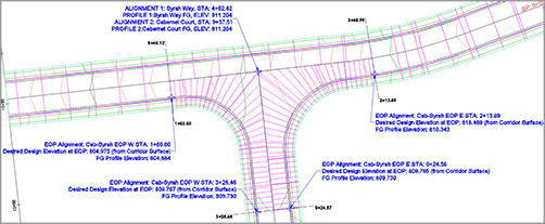
23. Once all the labels have been placed, confirm that your corridor looks like Figure 10-59.
Figure 10-59: The corridor with all labels placed
As you can observe from the labels, the profiles and the surface model are darn close. In fact, if the 0.1′ bust doesn’t bother you, you can skip the next steps. If you want your design to be as perfect as it can be, carry on:
1. Open the Manual Intersection_Adjustment.dwg file (which you can download from this book’s web page), or continue working in your drawing from the previous exercise.
2. If you continue working in the previous drawing, you will want to split your model space into two views for easier working. Change to the View tab and Set Viewports Two: Vertical. Press ↵ at the command line to specify a vertical split. Your screen should look similar to Figure 10-60.
Figure 10-60: Use a split screen to see the plan and profile simultaneously.

3. Pick the Cab-Syrah EOP W - FG profile (the blue line in the profile view). From the contextual Ribbon, click Geometry Editor.
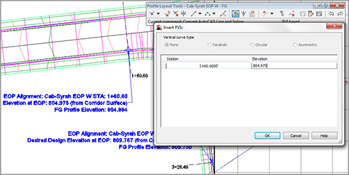
4. On the Profile Layout Tools toolbar, click Insert PVIs Tabular.
5. In the Insert PVIs dialog box, set the vertical curve type to None. Type 160.6 for the station. (Station notation is not needed.) Type 804.975 for the elevation. Click OK.
6. Select the corridor and choose Rebuild Corridor from the contextual tab. Your first curb return label will now report a perfect match between the Corridor Surface elevation and the FG Profile elevation (Figure 10-61).
Figure 10-61: Add PVI stations and elevations to match the desired FG elevations.
7. Repeat steps 3 through 5 for station 3+28.46 on Cab-Syrah EOP W - FG and station 2+13.69 on Cab-Syrah EOP E - FG (station 0+24.56 does not need this adjustment since it already happens to match perfectly).
8. Pick your corridor. Right-click and choose Object Viewer.
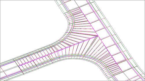
9. Navigate through the Object Viewer to confirm that your corridor model is now appropriately tied together at the EOP. Note that any changes in the centerline won’t automatically update your EOP alignments. Your corridor should look like Figure 10-62.
Figure 10-62: The properly modeled intersection
10. Exit the Object Viewer showing just the corridor and look at your surface. Pick the corridor surface, and use the Object Viewer to study the TIN in the intersection area.
Study the contours in the intersection area. You are not quite done perfecting the surface model, but you are getting close. In the next section you will learn about tools you can use to make the corridor surface model even more precise.
Refining a Corridor Surface
Once your model makes more sense, you can build a better corridor surface. At any time you can continue to edit, refine, and optimize your corridor as you gain new information—and because all the corridor elements are connected and labeled, it will take only a few minutes for any edits to be reflected in the corridor surface.
In this exercise, you’ll use links as breaklines and add feature lines. You may wish to review the section “Creating a Corridor Surface” in Chapter 9 that explains corridor surface models in more detail. When you’re building a surface from links, you have the option of selecting a check box in the Add As Breakline column. Doing so adds the actual link lines as additional breaklines to the surface. In most cases, especially intersection design, selecting this check box forces better triangulation.
In the next exercise, you’ll add a few meaningful corridor feature lines to the surface to force triangulation along important features like Edge Of Travel Way and Top Of Curb.
The more appropriate data you add to the surface definition, the better your surface (and therefore your contours) will look—right from the beginning, which means fewer edits and less grading by hand. Follow these steps:
1. Open the Manual Intersection_Refining.dwg file (which you can download from this book’s web page), or continue working in your drawing from the previous exercise.
2. Pick one of the contours from the corridor surface in the drawing. Click Surface Properties from the contextual Ribbon tab. The Surface Properties dialog opens.
3. Change Surface Style Of Corridor Surface to No Display so you don’t accidentally pick it when choosing a corridor boundary. Click OK to dismiss the dialog.
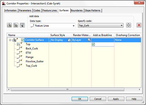
4. Select the corridor, and choose Corridor Properties from the contextual Ribbon tab. Switch to the Surfaces tab. In the row for the Top, under Corridor Surface, click the check box in the Add As Breakline column if it is not already checked.
5. Select Feature Lines from the drop-down menu in the Data Type selection box.
6. Use the drop-down menu in the Specify Code selection box and the + button to add the Back_Curb, ETW, Flange, Flowline_Gutter, and Top_Curb feature lines to the Corridor Surface, as shown in Figure 10-63.
Figure 10-63: Adding feature lines to the corridor surface
7. Click OK to dismiss the dialog, and your corridor will automatically rebuild, along with your corridor surface.
8. Select your corridor surface under the Surfaces branch in Prospector. Right-click and choose Surface Properties. The Surface Properties dialog opens. Change Surface Style to Contours 1′ and 5′ (Prop), and click OK. Click OK to dismiss the Surface Properties dialog.
You can make additional, optional edits to the TIN if you’re still unhappy with your road surface. Edits that may prove useful include increasing the corridor frequency in select regions, adjusting the start and end stations in a region, or using surface-editing commands to swap edges or delete points.
When Automatic Surface Boundaries Are Not Available
You will come to a point in the corridor modeling where you need to add a corridor surface boundary, but the best options (Add Automatically Daylight or Corridor Extents As Outer Boundary) are not available. There will also be situations where Corridor Extents As Outer Boundary does not go where you want it to go. In those situations, you will need to use the Add Interactively tool.
Add Interactively allows you to direct Civil 3D to use the correct feature line as the boundary. You will trace your desired outer bounds with a temporary graphic called a jig.
1. Open the Concord Commons Corridor.dwg file, which you can download from the book’s web page. You will see a surface in this file that needs some serious reining in.
2. Select the corridor, and click Corridor Properties on the contextual Ribbon. Select the Boundaries tab.
3. Right-click on the Concord Commons Corridor Top surface and select Corridor Extents as the outer boundary. Click OK.
Pan around the drawing. The contours are tidier, but the surface inside the loop formed by Frontenac Drive has not been cleaned up. In the next steps of the exercise, you will clean up the surface using the Add Interactively tool.
4. Set your AutoCAD object snaps to use only Endpoint and Nearest. These will be the most helpful osnaps to steer Civil 3D in the right direction.
5. Select the corridor and open the Corridor Properties dialog. On the Boundaries tab, right-click Corridor Boundary(1) and select Remove Boundary.
6. Right-click Concord Commons Corridor Top and select Add Interactively.
7. Start on the right side and click the Sidewalk_Out feature line. Trace it with your cursor. When the jig is going to the correct location, click to commit the boundary. The following image shows what the jig will look like:
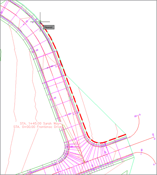
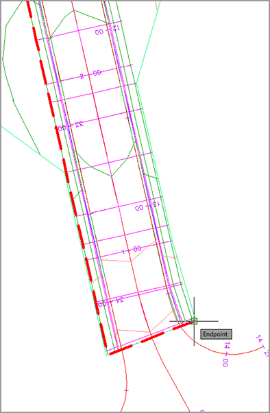
As you move around, you will see the jig tend to move unexpectedly at region boundaries. Steer the jig where you want it to go by clicking and tracing. If you made a mistake, type U for undo at the command line. When you reach a point where you need to cross a street, use the endpoint snap to jump the jig across, as shown here:
If you click a location where there is more than one feature line, or you are zoomed out to where your pickbox encompasses two lines, you will see a dialog like this one asking you to pick the line you are after:

8. After you have finally come back around to where you started the boundary, type C (for close) at the command line and press ↵.
9. Right-click on the name of the surface again. Select Add Interactively. This time, repeat the process for the inner boundary, again using the Sidewalk_Out feature line as the boundary.
10. When you complete the inner loop and return to the Corridor Properties dialog box, set the boundary type to Hide Boundary, as shown here.

Yes, this process can be tedious. However, your work will pay off when changes are made to your design. These boundaries are dynamic to the design, unlike a polyline boundary.