
Earthwork is a major part of almost every land development project. The money involved with earthmoving is a large part of the budget, and for this reason, minimizing this impact is a critical part of the final design. Civil 3D contains a number of surface analysis tools designed to help in this effort, and you’ll look at them in this section. First, a simple comparison provides feedback about the volumetric difference, and then a more detailed approach enables you to perform an analysis on this difference.
For years, civil engineers have performed earthwork using a section methodology. Sections were taken at some interval, and a plot was made of both the original surface and the proposed surface. Comparing adjacent sections and multiplying by the distance between them yields an end-area method of volumes that is generally considered acceptable. The main problem with this methodology is that it ignores the surfaces in the areas between sections. These areas could include areas of major change, introducing some level of error. In spite of this limitation, this method worked well with hand calculations, trading some accuracy for ease and speed.
With the advent of full-surface modeling, more precise methods became available. By analyzing both the existing and proposed surfaces, a volume calculation can be performed that is as good as the two surfaces. At every TIN vertex in both surfaces, a distance is measured vertically to the other surface. These delta amounts can then be used to create a third volume surface representing the difference between the surfaces. Civil 3D uses this methodology to perform its calculations, but the end-area method can still be used if desired.
Simple Volumes
When performing rough analysis, the total volume is the most important part. Once an acceptable volume has been created, more refined analysis and comparison can be performed. In this exercise, you’ll compare two surfaces to pull a basic volume number and then modify the proposed grade to illustrate how quickly changes can be reviewed:
1. Open the SurfaceVolumes.dwg file.

2. Change to the Analyze tab, and then click the Volumes button on the Volumes And Materials panel to display Panorama open to the Composite Volumes tab, as shown in Figure 4-43.
Figure 4-43: The Composite Volumes tab in Panorama
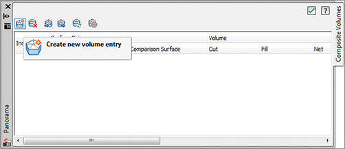
3. Click the Create New Volume Entry button on the far left, as indicated in Figure 4-43, to create a new volume entry.
4. Click the <select surface> field under the Base Surface heading and select EG.
5. Click the <select surface> field under the Comparison Surface heading and select FG. Civil 3D will calculate the volume (Figure 4-44). Note that you can apply a cut or fill factor by typing directly into the cells for these values.
Figure 4-44: Composite volume calculated

6. Without closing Panorama, move to Prospector, and expand the Surfaces FG Definition branches.
Don’t Touch That Close Button!
This utility’s calculations will disappear if you close Panorama. You can export this information to XML or copy and paste it into another document if you require a record.
7. Right-click Edits and select the Raise/Lower Surface option.
8. Enter –0.25 at the command line to drop the site 3″.
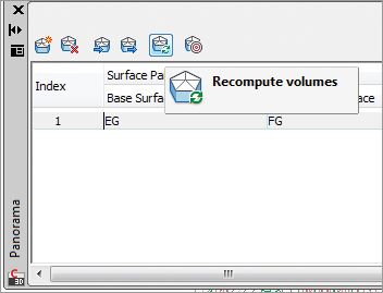
9. In Panorama, click the Recompute Volumes button (as shown in Figure 4-45) to update the calculations.
Figure 4-45: Recomputing the composite volume
10. Right-click the Edits list to remove the lowering edit and select Delete.
11. Return to Panorama and recompute to return to the original volume calculation.
The original design was quite good in terms of cut and fill, so in the next section you will look at a more detailed analysis of the earthwork by using a TIN volume surface.
Volume Surfaces
Using the volume utility for initial design checking is helpful, but quite often, contractors and other outside users want to see more information about the grading and earthwork for their own uses. This requirement typically falls into two categories: a cut-fill analysis showing colors or contours or a grid of cut-fill tick marks.
Color cut-fill maps are helpful when reviewing your site for the locations of movement. Some sites have areas of better material or can have areas where the cost of cut is prohibitive (such as rock). In this exercise, you’ll use three of the surface analysis methods to look at the areas for cut-fill on your site:
1. Open the SurfaceVolumes.dwg file if it is not already open.
2. In Prospector, right-click the Surfaces branch and select Create Surface. The Create Surface dialog appears.
3. Change the Type field to TIN Volume Surface.
4. Expand the Information property, and change the Name to Volume.
5. In the Style value field, click the ellipsis button to open the Select Surface Style dialog. Select Elevation Banding (2D) and click OK.
6. Expand the Volume Surfaces property, and click in the Base Surface value field. Click the ellipsis button to open the Select Base Surface dialog. Select EG and click OK.
7. Click in the Comparison Surface value field. Click the ellipsis button to open the Select Comparison Surface dialog. Select FG and click OK. Your screen should look like Figure 4-46. Note that you can apply cut and fill factors to your calculations by filling them in here.
Figure 4-46: Creating a volume surface

8. Click OK to complete the surface creation.
This new volume surface appears in Prospector’s Surfaces collection, but notice that the icon is slightly different, showing two surfaces stacked on each other. The color mapping currently shown is just a default set, though, and does not indicate much.
9. Right-click Volume in the Surfaces branch of the Prospector and select the Surface Properties option. The Surface Properties dialog appears.
10. Switch to the Statistics tab and expand the Volume branch.
The value shown for the Net Volume (Unadjusted) is what was calculated in the Surface Volume utility in the previous exercise. This information can be cut and pasted into other programs for saving or other analysis if needed.
11. Switch to the Analysis tab.
12. Change the Number field in the Ranges area to 3, and click the Run Analysis arrow.
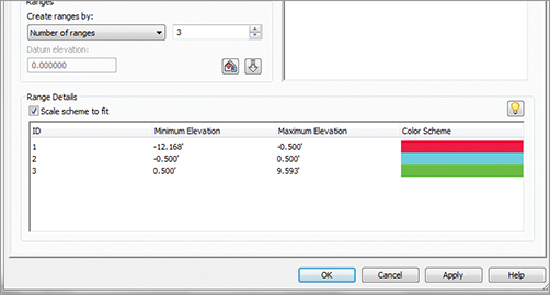
13. Change the values in the cells by double-clicking and editing to match Figure 4-47. The colors that would be recommended are red, cyan, and green, where red indicates the worst case cut, green represents the worst case fill, and cyan represents a balance.
Figure 4-47: Elevation analysis settings for earthworks
14. Click OK to close the dialog.
The volume surface now indicates areas of cut, fill, and areas near balancing, similar to Figure 4-48. If you leave a small range near the balance line, you can more clearly see the areas that are being left nearly undisturbed.
Figure 4-48: Completed elevation analysis

To show where large amounts of cut or fill could incur additional cost (such as compaction or excavation protection), you would simply modify the analysis range as required.
The Elevation Banding surface is great for onscreen analysis, but the color fills make it hard to plot or use in many applications. In this next exercise, you use the Contour Analysis tool to prepare cut-fill contours in these same colors:
1. Right-click Volume in the Surfaces collection of Prospector and select the Surface Properties option to open the Surface Properties dialog again.
2. On the Analysis tab, set the Analysis Type field to Contours.
3. Change the Number field in the Ranges area to 3.
4. Click the Run Analysis button.
5. Change the ranges as shown in Figure 5-44. The contour colors are shades of red for cut, a yellow for the balance line, and shades of green for the fill areas. Click the small button to display the AutoCAD Select Color dialog.
6. Switch to the Information tab on the Surface Properties dialog, and change the Surface Style to Contours 1″ and 5″ (Design).
7. Click the down arrow next to the Style field and select the Copy Current Selection option. The Surface Style Editor appears.
8. On the Information tab, change the Name field to Contours 1″ and 5″ (Earthworks).
9. Switch to the Contours tab.
10. Expand the Contour Ranges branch.
11. Change the value of the Use Color Scheme property to True. It’s safe to ignore the values here because you hard-coded the values in your surface properties.
12. Click OK to close the Surface Style Editor and click OK again to close the Surface Properties dialog.
The volume surface can now be labeled using the surface-labeling functions, which you’ll look at in the “Labeling the Surface′ section.
To expand on the Elevation Banding surface, we can now automate the process. Say we needed to show the contractor a drawing showing elevation changes in our volume surface, but at 2′ intervals.
The old way would have been to assign elevations, and manually change the minimum and maximum elevations and the associated colors.
New to Civil 3D 2012, we now have the capability to set either a range interval or range interval with datum. Let’s take a look at how this works:
1. While still in SurfaceVolumes.dwg, click on the volume surface and select Surface Properties from the Modify panel.
2. Click on the Analysis tab and under the Create Ranges By drop-down, you now have the Range Interval and Range Interval with Datum. Select the Range Interval with Datum option.
3. Set the interval to 2, for 2′ contour range intervals.
4. Click on the Run Analysis button and click OK.
The surface is now colorized with a range of colors representing the 2′ contour intervals for the elevations.
Another Volume Option—Bounded Volumes
The Bounded Volumes tool is very useful for checking volumes for a smaller area. In this example, the developer wants to know the volume of a single lot in order to start developing.
1. Open the BoundedVolumes.dwg file. This is the overall drawing, but has a thick polyline around the boundaries of Lot 4.
2. From the Modify tab and Ground Data panel, select Surface.
3. From the Surface tab and Extended Analyze tab, select Bounded Volumes.
4. Press ↵ and select the Volume surface.
5. Select the thick polyline around the perimeter of Lot 4.
6. Press ↵ to end the command.
7. Press F2 to see the volume report for Lot 4.
You can see that the volume for Lot 4 is a Net cut of 535 cubic yards.
You can also use this tool if you wish to set a datum elevation for a non-volume surface, such as establishing a grading pad for a building.