
Since Civil 3D is built upon Map 3D, we would be remiss if we didn’t mention its existence and some of its features. An entire book could be written on this subject, so only the basic parts and how they pertain to Civil 3D will be discussed here.
Map 3D is the geographical information system (GIS) part of Civil 3D. It lies there ready and willing to jump in and help you out. Still, many people don’t know about its existence. Hold on to your hats for a whirlwind tour of Map 3D.
Where Is It?
Out of the box, Civil 3D starts up with a workspace called Civil 3D. This workspace contains all the tools necessary to work on Civil 3D. Down on the status bar, you will find the Workspace switcher. The flyout workspace choices are:
- Civil 3D
- 2D Drafting & Annotation
- 3D Modeling
- Planning And Analysis Workspace
The last option (Planning And Analysis Workspace) is the Map 3D Workspace. Clicking that option will transform your screen into the new tools on the tabs and panels shown in Figure 17-35.
Figure 17-35: The Planning and Analysis Workspace

Setup
To efficiently use Map 3D, you need to do some housework, such as a creating a drive alias and attaching drawing files. So let’s get to it.
Drive Alias
The ability to attach drawings and other objects is invaluable to Civil 3D so that you can load only what you want to. To assist in this effort, setting up drive aliases will make life a bit easier for you. You can liken a drive alias to data shortcuts (which we covered earlier this chapter). Here’s the procedure:
1. Start a new drawing using any template you wish.
2. Using the Workspace switcher (located at the bottom of your drawing screen), select Planning And Analysis Workspace. This switches the workspace to the Map 3D with its associated tabs and panels.
3. From the Data panel on the Home tab, select the Attach tool. The Select Drawings To Attach dialog opens.
4. Click the Create/Edit Alias icon. The Drive Alias Administration dialog opens. Here is where you will set an alias and the path to it.
5. In the Drive Alias Details section, type Mastering in the Drive Alias text box. Click the Browse button and navigate to the C:Mastering folder and click OK.
6. Back in the Drive Alias Administration dialog, click the Add button, as shown in Figure 17-36. Click Close. If an error message pops up, close it. The alias has been saved, as shown in Figure 17-37. You can repeat this process for as many aliases you want. Click OK to close this dialog.
Figure 17-36: The Drive Alias Administration dialog
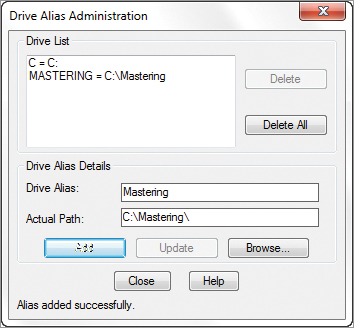
Figure 17-37: The Select Drawings To Attach dialog

7. You can now copy your GIS files to this new location. Locate the GIS folder, which you can download from this book’s web page. Copy the GIS folder and all of its contents into the C:Mastering folder. (You could have also done this step before creating the drive alias).
Attach Drawings
Now that you have a drive alias (or multiple aliases) set up, you can attach drawing files to your empty drawing. These drawings are not just regular AutoCAD drawings; they contain features that you will pull from later. So, let’s attach a drawing:
1. Reopen the Select Drawings To Attach dialog by clicking the Attach tool on the Data panel of the Home tab.
2. In the Look In section, use the drop-down list box to select your aliased drive. Note that the author’s alias is pointing to a larger drive where the GIS data is stored. This brings up a good point: You could alias a location on the server for these objects since many of them can be quite large in size.
3. Double-click the Counties folder, select the US Counties object, click Add, and then click OK. Yes, you select US Counties even though you are dealing with only a portion of a county. This way, you can see how powerful the query options are in Map 3D that will be covered later.
4. The counties drawing has been attached, but nothing is showing on the screen. This is because, although the drawing is loaded, it is not visible. Another way to think about this is you do not want to see every county in the United States on your drawing. You want to look inside that drawing and pull out the data that you really need to see, which we will cover next.
Queries
This section is one of the most powerful reasons to learn about 3D Map: the ability to pull data from different sources (such as SHP files) and come up with a drawing to just show those.
1. In the Task pane, select the Data tool.
2. From the flyout menu, select Connect To Data. The Data Connect palette opens.
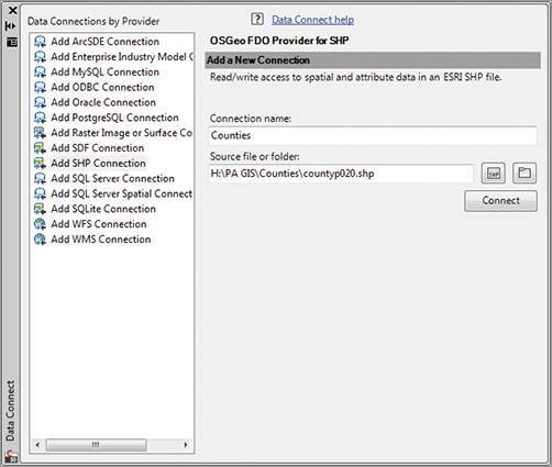
3. Click the SHP icon, navigate to the Counties folder, and select the countyp020.shp file.
4. Type Counties in the Connection Name text box. Your palette should look similar to Figure 17-38. Click Connect.
Figure 17-38: The completed Data Connect palette
5. In the Data Connect palette, click the Add To Map flyout and select Add To Map With Query. The Create Query wizard opens.

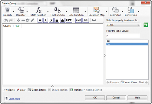
6. You want to find York County in the state of Pennsylvania, so you will start large and narrow down. Click the Property tool and select State.
7. Click the Equals tool.
8. Click the Get Values tool, and in the filter box, type the letter P. This sets the filter to all states that begin with the letter P. Click the green button and then select PA from the list. You could have simply selected the green arrow and then scrolled to find Pennsylvania, but we wanted to show you the power of the filter.
9. Click the Insert Value tool. Your query thus far looks like Figure 17-39.
Figure 17-39: The query thus far

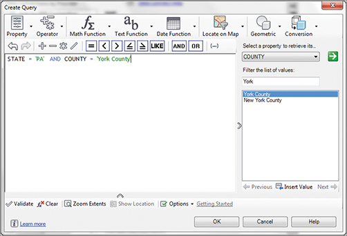
10. We need to add to the query by finding York County within the state of Pennsylvania. Click the Operator tool and select AND. This is a logical operator that means all conditions must be met in order to find a match.
11. Repeat steps 5–7 but look for the Property to query COUNTY and the value to query York County, as shown in Figure 17-40. Click OK.
Figure 17-40: The finished query
12. Perform a zoom extents. Only the polygon for York County, Pennsylvania is displayed, although there are over 3,000 to choose from. In addition, there are five counties in the United States that are York County.
13. Save your drawing as GISMAP.dwg.
Hopefully, you can see the power of Map 3D and how you can create custom reports like the following:
- What properties are affected by the proposed 50′ right-of-way that is going in on the highway?
- How many red maple (Acer Rubrum) trees are on your 36-acre lot?
- You need a coverage report of fire hydrants based off a cityscape, keeping in mind that hoses cannot go through buildings.
So you can see that the possibilities are pretty much endless as long as you have valid data, which can be procured from your municipal GIS department or even on the Internet.
Scratching the Surface
No, we have not gone in-depth at all with Map 3D—we haven’t even scratched the surface! There could be books that would equal the size of this book just on the subject of Map 3D.
If our little exercise piqued your curiosity about Map 3D, then our object was fulfilled. Luckily, resources are available to help you learn more about the subject.
One such resource comes from James Murphy, who many consider to be a Map 3D guru. His blog, Map 3D and Murph’s Law (map3d.wordpress.com), is a great source for Map 3D.
Don’t forget the help and tutorials that are included with Civil 3D. As we mentioned earlier, Civil 3D is built on Map 3D and the help/tutorials are included with your Civil 3D.