
SSA can perform a number of water- and wastewater-related tasks. In the remainder of this chapter, you will be going through several examples of what SSA can do, but you are just seeing the tip of the proverbial iceberg.
In the next section, you will focus on the workflow between Civil 3D and SSA.
In the following section, you will learn how to create subbasins (catchments) directly in SSA. You’ll also see examples of the Rational method and TR-55 and learn about SSA reports.
Guided Tour of SSA
SSA is not at all like AutoCAD. It is a true modeling software that shows a schematic of your design in a plan view. On the left side of the screen you will see the data tree. Like Prospector in Civil 3D, the SSA data tree gives you access to tools and information about objects.
The easiest way to add new structures, pipes, or catchments to the project is to do so from the Elements toolbar along the top of the screen. Here you will find everything you need to build a project from scratch if you did not start out in Civil 3D.
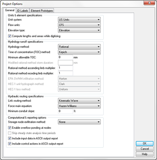
The next stop on our tour is the Project Options dialog (Figure 14-10). Access Project Options by double-clicking on the listing in the data tree. Project Options is where you set your units, hydrology method, routing method, and force main equation. Depending on the scope of your project, you may not need to worry about every equation used. In the following example, you will use the Rational method with TR-55 Tc calculations. Since you are calculating runoff only, you do not need to set the other project options. Once you have finished entering the options shown in Figure 14-10, click OK.
Figure 14-10: SSA Project Options dialog

Whenever you are designing in SSA, always work upstream to downstream. If your system includes a pump, you should work from highest elevation to lower elevations.
An SSA project consists of three main object types: subbasins, nodes, and links:
Subbasins Subbasins are important for runoff computations but are not mandatory if you are inputting flows manually. Subbasins can be defined directly in SSA or brought over as data from Civil 3D. SSA can also turn an SHP file directly into a subbasin.
Nodes Nodes are the workhorses of SSA, and can take several forms:
Junction Node Nodes are where all calculations are done in SSA. If you want information along a pipe, for example, you will need to place a junction node at the location of interest. These can be used as null structures, water, or pollutant infiltration points.
Outfall Node Outfall node is the end of your system. An outfall can be where proposed sewer ties into existing, where sanitary sewer enters a treatment facility or a culvert discharge location. An outfall can be attached to only one link.
Flow Diversion Node If a node has two outgoing links, you will need to use a flow diversion. Flow diversions most commonly represent multiple outflow points on a detention basin, such as a weir or orifice. They can also represent flow diversion in a combined sewer system or anywhere an overflow check is in use.
Inlets When SSA converts structures from Civil 3D, it assumes an inlet node by default. Inlets are used in storm systems and can collect flow from a subbasin. You can also manually enter flows.
Storage Nodes Anywhere water is detained on your site, a storage node can model the scenario. Storage nodes can represent ponds, wet wells, underground storage, or a residential rain barrel.
Links Links connect nodes to each other. Links represent pipes, channels, curbs, and gutters, or culverts.
Hydraflow, We Haven’t Forgotten You
When it comes to flexibility in storm design and routing, SSA beats the pants off of Hydraflow any day. In general, there is a lot of overlap between the two products. For basic storm sewer calculations, either product will work great. When your designs get more complex and require hydrograph and storage routing with infiltration and exfiltration, SSA has a much better solution.
You can still access all the Hydraflow functions from the Analyze tab Design panel flyout.

Hydraflow is still part of the picture when it comes to exporting and importing data to and from Civil 3D. Hydraflow’s file format does a much better job than LandXML at keeping the data integrity of your pipes and structures.
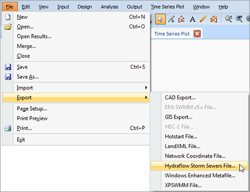
When exporting from SSA, choose File Export Hydraflow Storm Sewers File for the best path back to Civil 3D.
Hydrology Methods
SSA is capable of computing rainfall runoff using any of the following methods:
Rational Method The Rational method is used to approximate the peak discharge (or flow, Q) from an impervious area (A) using the tried and true Q=ciA. This is the most common method used for sizing sewer pipes.
Imagine yourself outside in a rainstorm, staring at a single point on your driveway (assuming your driveway is impervious and on a nice, even slope). At first, the water on your driveway is coming right from the sky. After a while, water flows in from rain falling elsewhere in your neighborhood. Now imagine that the storm stops as soon as raindrops from the farthest point in your neighborhood reach the point on your driveway.
The Rational method is based on the assumption that it takes the same amount of time for those farthest raindrops to get to you as they do to run off your driveway completely.
The first step to using the Rational method is to delineate the drainage basin, as described earlier in this chapter, and assign composite runoff coefficients. SSA needs an intensity-duration-frequency (IDF) curve for the study area to compute the rainfall.
Modified Rational and DeKalb Rational These hydrology methods are similar to the Rational method, except that they are intended to approximate the storage volume needed on small, simple detention basins. Instead of the storm duration equaling two times the time of concentration, the storm duration is longer. The longer storm duration results in a larger volume than the Rational method but results in a lower peak discharge.
The same information is needed for the Modified and DeKalb Rational methods as for the Rational method, and you must have a value in the Project Options dialog for Modified Rational Storm Duration.
Both the Rational method and the Modified Rational method are intended for small watersheds, usually less than 20 acres (8.1 hectares).
SCS TR-55 Method and TR-20 Method More gifts from the USDA, the SCS TR-55 runoff method is a more complex method that is appropriate for study areas up to 2,000 acres (809 hectares).
For the SCS TR-55 and TR-20 methods, SSA contains tools for looking up computation variables. You will find a curve number (CN) lookup table inside the subbasin. SSA will even help you determine the composite curve number. The TR-55 hydrology method is also where you will use SSA rain gauges.
HEC-1 The US Army Corps of Engineers’ Hydraulic Engineering Center has a computer program called HEC-1 for hydrology calculations. The HEC-1 method in SSA duplicates the results from the Army Corps’ program. Their method is used in situations where there is an existing body of water, such as a stream. For an explanation of this method directly from the source, go to http://www.hec.usace.army.mil/publications/TrainingDocuments/TD-15.pdf.
EPA-SWMM The US Environmental Protection Agency (EPA) Storm Water Management Model (SWMM) method is used for developed watershed areas and can take into account many more factors than the other analysis methods. SWMM allows for localized ponding effects, which can be entered into the subbasin physical properties area. This method also allows for the effects of existing soil moisture, evaporation, and snowmelt in the system. When using EPA-SWMM, be sure to set all the methods you intend to use for infiltration and exfiltration in the Project Options dialog.
A Few Hints for Working in SSA
Since this is not traditional CAD, the program behaves differently than you might expect. This list contains a few hints to help you along the way:
- Make sure you download and install the Civil 3D 32-bit object enabler. SSA needs the object enabler to see Civil 3D objects such as pipes, structures, and nodes. Since SSA is a 32-bit application under the hood, download the 32-bit version of the object enabler even if your computer is on a 64-bit operating system.
- Unlike AutoCAD, SSA keeps you in a command until you press Esc, or click the Select Element tool from the toolbar.
- Another “gotcha” are the tabs along the top of the screen. To dismiss them, use the red X that appears on the tab itself. It is a common mistake to dismiss the program accidentally by clicking the incorrect red X.

- Don’t forget to save! Unlike CAD, there is no auto-save.
- Also, there is no Undo command in SSA. Luckily, adding and removing elements is a simple process. If something gets goofed up beyond repair, you could always close without saving.
It may take a while to get used to, but SSA is a powerhouse analysis tool.
In the following example, you will work through a simplified example to get the feel for the SSA interface:
1. Launch SSA from the stand-alone icon in your computer’s Start menu. This will launch SSA with an empty project.
2. In the SSA interface, choose File Import Layer Manager (DWG/DXF/TIF/more), as shown in Figure 14-11. Click the ellipsis next to the Image/CAD File field. Browse to the file SSA Intro.dwg, which you can download from this book’s web page. Place a check mark next to Watermark Image and click OK.
Figure 14-11: To show the AutoCAD information as an underlay, import it as a background layer

When you import the CAD file, make a mental note of the many file formats that can be used to import data to SSA, including EPA SWMM.
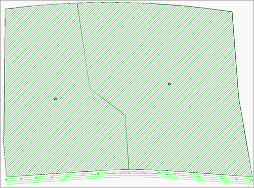
3. Click the green Add Subbasin button from the elements toolbar along the top of the window. Using this tool, click around the boundary lines that represent the example watersheds. When you are close to completing a shape, you can right-click and select Done to close the shape.
There are no snap or curve drawing tools in SSA. Digitize as closely as possible using multiple small segments. If you make a mistake, you can right-click and select Delete Last Segment. Later on in this chapter we will look more closely at modifying vertices of a completed shape.
4. When you have completed both shapes, your graphic will resemble Figure 14-12.
Figure 14-12: New subbasins in SSA
5. Switch to the Inlet tool by clicking the Inlet button at the top of the SSA window.
6. Place two inlets on the south side of the site. An X has been placed at each inlet location to help you locate the recommended positions.
When you have finished placing inlets, press Esc on your keyboard or click the arrow icon in SSA to get back to Selection mode. If you accidentally place more inlets than you wanted, you can right-click the wayward inlet while in Selection mode and select Delete from the menu.
7. Click the Outfall icon. Click to place the outfall structure in the location marked with a circle at the southeastern corner of the site.
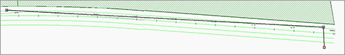
8. Next, switch to the Conveyance Link tool. Working from left to right across the project, click the upstream inlet. Resist the temptation to click and drag. Connect the first inlet with a straight segment to the second inlet. Next, connect the second inlet to the outfall. At this point your SSA file should resemble Figure 14-13.
Figure 14-13: Pipes connecting inlets to each other and the outfall
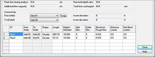
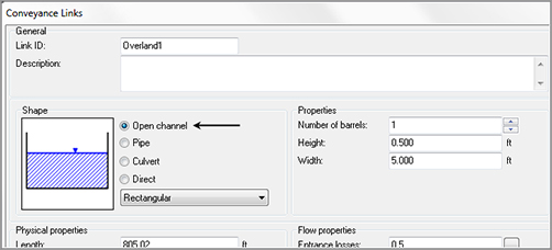
9. Double-click the first conveyance link you created. You will see the Conveyance Links dialog. The easiest place to rename the pipes is in the small grid at the bottom of the box, as shown in Figure 14-14. When your cursor is in the field to rename a pipe, a dark black square will appear on the pipe in the main graphic, helping to indicate which pipe you are editing. Rename the first link to Pipe1. Rename the second conveyance link to Pipe2.
Figure 14-14: The Conveyance Links dialog is the main pipe and channel control tool.
So far, you’ve told SSA what your drainage areas are and you’ve established a pipe network. Next, you need to tell SSA which subbasin drains to which inlet.
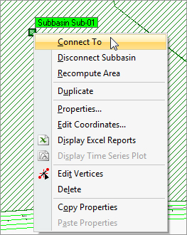
10. Switch to the selection tool by pressing Esc if it is not already active. Right-click the icon that represents the western subbasin and select Connect To, as shown in Figure 14-15.
Figure 14-15: Connecting a subbasin to an inlet
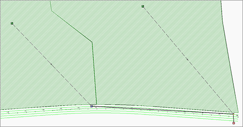
11. Connect the subbasin to the western inlet (Inlet-01) by clicking the inlet symbol in plan view. A line will form to indicate the connection was successfully created. Repeat the process for the eastern subbasin and inlet (Inlet-02). At the end of the process your SSA screen will resemble Figure 14-16.
Figure 14-16: Subbasins assigned to inlets
Before SSA can run any analysis on the project, you must make one last crucial connection. Both of these inlets are on grade, which means water will flow toward them, but in a big storm, some water may flow past into the next downstream inlet. The flow along the gutter of the road between inlets is called a bypass link.
12. Click the Add Conveyance Link button. Connect Inlet-01 to Inlet-02 again, but this time follow the curve of the road. This conveyance link represents the gutter flow of any water that doesn’t make it into Inlet-01 and continues on to Inlet-02.
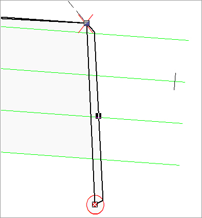
13. Add a conveyance link between Inlet-02 and the outfall. To visually differentiate the culvert from the bypass link, you can put a small kink in the line, as shown in Figure 14-17. When you modify link properties, you will have the opportunity to compensate for the change in length this technique causes.
Figure 14-17: The bypass link between Inlet-02 and the outfall
14. Rename the new links to Overland1 and Overland2, respectively.
All the pieces are here; next you will assign elevations to the pipes, inlets, outfalls, and curb flows.
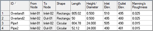
15. Double-click any of the links to open the Conveyance Link dialog. Using the tabular input at the bottom screen, key in the values for Diameter, Inlet Elevation, Outlet Elevation, and Manning’s Roughness, as shown in Figure 14-18.
Figure 14-18: Set pipe and gutter elevation data as shown.
16. For the overland flow links, you will use a rectangular open channel to approximate gutter flow. For both Overland1 and Overland2 links, set the width to 2′, as shown in Figure 14-19. Click Close when complete.
Figure 14-19: Set the channel type and width as shown.
17. Next, you will set the Inlet elevations by double-clicking on Inlet-01.
- Using the Inlets dialog, set the number of inlets for both Inlet-01and Inlet-02 to 2, as shown toward the top of Figure 14-20.
Figure 14-20: Setting Invert Elevation and design settings
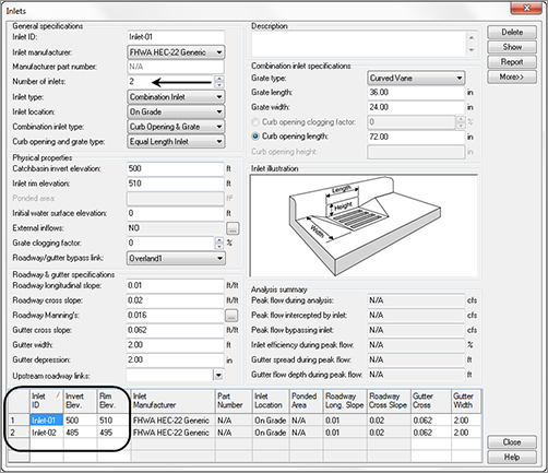
- Set Invert Elevation and Rim Elevations, as shown at the bottom of Figure 14-20.
- For Inlet-01, set Roadway/Gutter Bypass Link to Overland1, as shown in Figure 14-20.
- For Inlet-02, set Roadway/Gutter Bypass Link to Overland2.
- Click Close when complete.
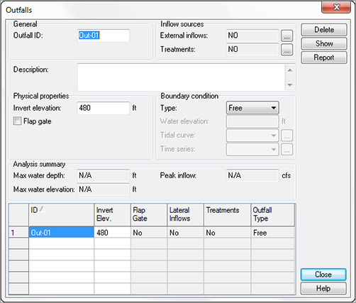
18. Double-click the Outfall location. Set the Outfall elevation to 480, as shown in Figure 14-21. Under Boundary Condition, set Type to Free. Click Close.
Figure 14-21: Outfall elevation and settings
Now that all the elevations are set, you must tell SSA how much rain you expect to see in your system.
19. In the data tree on the left side of the SSA window, click IDF Curves, as shown in Figure 14-22.
Figure 14-22: IDF Curves are found in the data tree.

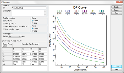
20. Click Load. Browse to the file York Co PA.idfdb. This is the rainfall data for our example file. After loading the file, set the ID to York, PA, USA, as shown in Figure 14-23. Click Close.
Figure 14-23: IDF curves entered in SSA
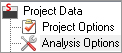
21. In the data tree on the far left, double-click Project Options. (This dialog takes a moment to open.)
- Set Hydrology Method to Rational.
- Set Time Of Concentration (TOC) Method to Kirpich.
Your Project Options dialog should resemble Figure 14-24. Click OK.
Figure 14-24: Verify your settings and click OK.
22. Double-click Analysis Options from the data tree.
- On the General tab, set the End Analysis On value to 02:00:00. Your dates will vary from what is shown in Figure 14-25, but the important thing is that the duration of the analysis is large enough to accommodate the Rational method.
Figure 14-25: Setting the design storm in Analysis Options
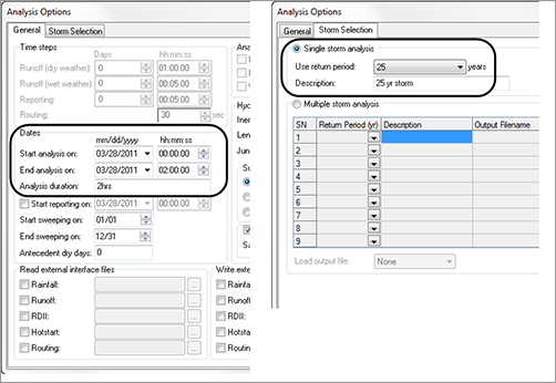
- On the Storm Selection tab, set Return Period to 25 years for a single storm analysis.
- Click OK when complete.
The last step before you are ready to run the design is setting the subbasin information for use with the Kirpich method of time of concentration. The Kirpich method calculates Tc based on the average slope and area characteristics of the site.
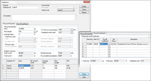
23. Double-click the green subbasin icon located in the centroid of the western subbasin.
- For the western subbasin, set the flow length to 750, and set the average slope to 3%.
- Switch to the Runoff Coefficient tab and set the runoff coefficient to 0.37.
- Switch to the eastern subbasin by selecting its row at the bottom of the dialog.
- Set the eastern subbasin flow length to 700, and set its average slope to 2.5%.
- When your dialog resembles Figure 14-26, click Close.
Figure 14-26: Final preparation of the subbasin data
24. Click Perform Analysis. After a moment, the analysis will complete. Click OK.
In the SSA graphic, you will see that conveyance link Overland1 is flooded. Later on in the chapter you will look at reporting capabilities to see details of this predicament.
25. Save the file as SSA Intro.spf.
From Civil 3D, with Love
Earlier in this chapter, you saw some of the preparations that must take place before you click the Edit In Storm And Sanitary Analysis button. Once inside SSA, a few more pieces of information need to be added before SSA can do its analysis.
In the following example, you will see what becomes of catchment objects and pipes once they are imported into SSA:
1. From Civil 3D, open the file C3DtoSSA.dwg. You can download this file from this book’s web page.
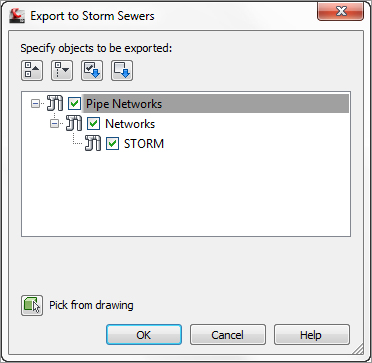
2. On the Design panel of the Analysis tab, click Edit In Storm And Sanitary Analysis. Verify that there is a checkmark next to the STORM network. Click OK in the Export To Storm Sewers dialog, as shown in Figure 14-27.
Figure 14-27: The pipe network on its way to SSA.
3. SSA launches. Click OK to create a new project. After a moment, SSA will let you know that you have successfully imported the Hydraflow Storm Sewers file. Click No, as you do not need to save the log file.
4. At the top of the SSA window, click Plan View. Examine the inlets and catch basins that have been imported.
Notice that an offsite outfall has been added to each inlet. This is because you don’t model the overland links in Civil 3D. When inlets are first imported into SSA, the program assumes they are on grade. Water that bypasses on grade inlets needs to go somewhere, so SSA automatically throws in an outfall to take care of the excess water. In the next steps you will remove the outfalls and create the overland links.
5. Right-click on the outfall that has been added to Structure 1. Click Delete, as shown in Figure 14-28. Click OK to confirm the deletion.
Figure 14-28: Right-click and click Delete to remove the extraneous outfall.
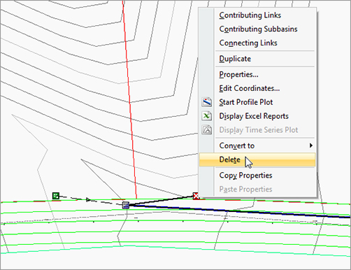
6. Right-click and delete the outfall to the far right.
7. Add overland conveyance links similar to the previous exercise. Add a link between Inlet Structure 1 and Inlet Structure 2. Add a link between Inlet Structure 2 and the outfall.
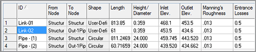
8. Double-click one of the conveyance links to edit the links in tabular form. Set the pipe and link design values as shown in Figure 14-29.
Figure 14-29: Design values for links and pipes
9. For the overland links, change the channel type to Open Channel. Set the shape type to User-Defined, as shown in Figure 14-30.
Figure 14-30: Gutter slope in cross-section; this will be the overland channel shape.
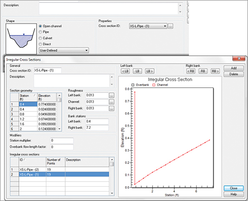
10. Click the ellipsis next to Cross-Section ID to open the Irregular Cross Sections dialog.
The shape you see in Figure 14-30 is an exaggerated view of a curb and gutter. In the previous example, you approximated the curb and gutter channel using a rectangular open channel. In this exercise, you will use one of the cross sections created for you by the export process.
11. For the active Cross Section ID, enter XS-L-Pipe - (1) and then click Close. Make sure both Links 01 and 02 are using the XS-L-Pipe (1) cross section for open channel flow. Click Close when your conveyance links are complete.
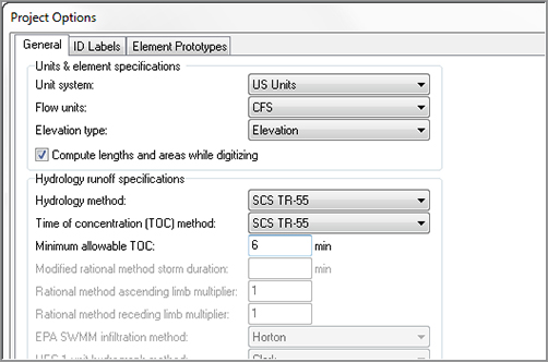
12. Double-click Project Options in the data tree. Set the Hydrology method to SCS TR-55. Set the Time Of Concentration method to SCS TR-55. Set Minimum Allowable TOC to 6 minutes. At the end of this step, your Project Options dialog should look like Figure 14-31.Click OK.
Figure 14-31: Project Options for this example
13. Back in the graphic, double-click the west subbasin. Switch to the SCS TR-55 TOC tab. You will input the following information to compute TOC for the western subbasin:
- On the Sheet Flow tab, set the Manning’s roughness value to 0.17.
This value is based off the TR-55 listing for different land conditions. The listing of values can be found by selecting the ellipsis next to the entry field.
- Set Flow Length to 150′.
This value is a site-specific measurement. Remember that in TR-55 sheet flow is considered to turn into shallow concentrated flow after 200′.
- Set Slope to 5%.
This is another site-specific value and represents the average overall slope of the subbasin.
- Click the ellipsis next to the 2Yr-24Hr Rainfall and in the resulting dialog, choose Pennsylvania from the State drop-down and York from the County drop-down, as shown in Figure 14-32. Click OK.
Figure 14-32: Sheet Flow input and rainfall location
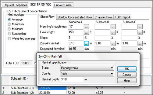
Selecting the rainfall location at this point is helping you determine the Tc. Your actual design storm duration may vary. Later in this chapter you’ll learn how rainfall works.
- Switch to the Shallow Concentrated Flow tab. Set Flow Length to 250′.
- Set Slope to 5%.
- Set the surface type to Short Grass Pasture.
The velocity for sheet flow will calculate based off the nomograph, which you can examine by clicking the ellipsis button next to Velocity. Your results should resemble the top of Figure 14-33.
Figure 14-33: Shallow concentrated flow and channel flow for TR-55

- Switch to the Channel Flow tab and set the Manning’s roughness value to 0.05.
- Set the flow length to 433′.
- Set the channel slope to 3%.
- Set Cross Section Area to 14.5.
- Set Wetted Perimeter to 12.2′.
Wetted Perimeter and Cross Section Area are site-specific values and are needed to calculate the hydraulic radius used in the Manning’s roughness equation. Figure 14-34 shows a schematic of what these values mean in channel flow.
Figure 14-34: The Cross Section Area and Wetted Perimeter values are used to find the Tc for channel flow.

After entering the values for channel flow, your dialog will now resemble the bottom of Figure 14-34.
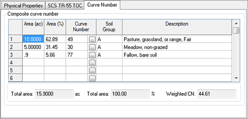
14. Still working with Sub-Structure - (1), switch to the Curve Number tab. Set the curve number values for the subbasin as shown in Figure 14-35.
Figure 14-35: Use these values on the Curve Number tab to create a weighted curve number.
15. Switch to the eastern subbasin by highlighting Sub-structure- (2) in the tabular listing. The Tc parameters for this subbasin are:
- Sheet Flow: Manning’s roughness of 0.17, Flow Length of 200′, and Slope of 4.5%.
- Shallow Concentrated Flow: Flow Length of 612′, Slope of 4%, Surface Type set to Short Grass Pasture.
- Channel Flow: Manning’s Roughness of 0.05, Flow Length of 305, Channel Slope of 2%, Cross Section Area of 12.2′, Wetted Perimeter of 8.4′.
16. Still working with Sub-Structure - (2), switch to the Curve Number tab and set the curve number to 45 for the entire area.
17. Click Close. Save the file as C3DtoSSA.spf for use in the next exercise.
Make It Rain
There are several methods for telling SSA the rainfall information for the model. A typical rainfall event in Herten, the Netherlands, is going to be vastly different from Arizona.
In the previous exercise, you set up many of the physical characteristics of the hydrologic system. You did not, however, tell SSA what type of rain to expect on the site.
Different hydrology methods require different assumptions about rainfall. In the Rational method, you used an intensity-based rainfall model (IDF Curve) because you were primarily interested in peak runoff. Because this is a TR-55 example, you will need to use rainfall information appropriate for this method.
1. Continue working in the file from the previous exercise or open SSA-Rain.spf in the Storm And Sanitary Analysis program. You can download this file from this book’s web page.
2. From the top of the SSA screen, select Add Rain Gauge. Click anywhere in the graphic to place the rain gauge in the project. Press Esc on your keyboard to return to Selection mode.
3. Double-click the New Rain gauge. Rename the Rain Gauge to Design Storm. Set Rain Data Format Type to Intensity. Set Incremental Interval to 0:20. At this step your Rain Gauge dialog will look like Figure 14-36.
Figure 14-36: The Rain Gauge dialog
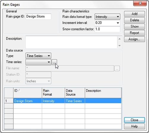
4. Click the ellipsis next to Time Series.
5. In the Time Series dialog, click Add. Rename the Time Series to York, PA 50.
6. Set the data type to Standard Rainfall and click the Rainfall Designer button.
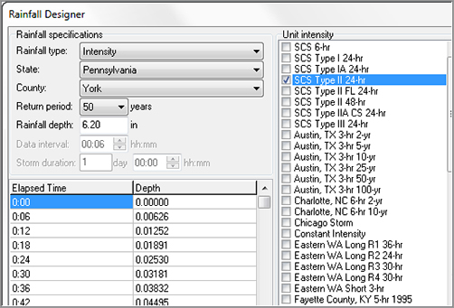
7. Set Rainfall Type to Intensity. Set State to Pennsylvania and County to York. Set Return Period to 50 years.
8. Make sure that the Unit intensity check mark is set to SCS Type II 24-hour, as shown in Figure 14-37. Click OK.
Figure 14-37: Rainfall Designer dialog
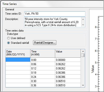
9. Once your Time Series dialog resembles Figure 14-38, click Close.
Figure 14-38: The completed time series
10. In the Rain Gauge dialog, click Assign. Click Yes when asked if you’d like to assign the rain gauge to all subbasins. Close the Rain Gauge dialog.
11. Double-click Inlet Structure - (1). Set Roadway Gutter Bypass Link to Link-01. Switch to Structure - (2) by selecting it from the table at the bottom of the Inlets dialog. Set Roadway Gutter Bypass Link to Link-02. Click Close.
12. Double-click Analysis Options on the data tree.
13. On the General tab, set the Analysis Duration to 1d by changing the date in the End Analysis On field to one day after the Start Analysis On (the exact date will vary depending on when you open the file).
14. On the Storm Selection tab, set Single Storm to Use Assigned Rain Gauge. Click OK.
15. Click Perform Analysis.
Running Reports from SSA
There are many places in SSA to view the results of your work. After you’ve run the analysis, the link and node listing will tell you if your pipe is underdesigned or if there is water backing up in the manholes.
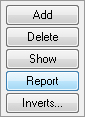
From virtually every dialog in SSA, clicking the Report button will create an Excel spreadsheet from the data you are observing. You will see the Report button for links, nodes, junctions, outfalls, and subbasins.
After running the analysis, you will want to see performance information and graphical representations of the relationship between the parts of your design. The Reports toolbar is at the top of the SSA screen. Figure 14-39 shows the different types of reports that you can choose.
Figure 14-39: The Reports toolbar
First, we’ll take a look at the hydrograph that has been created for the site.
1. From SSA, open the file SSA-Reports.spf. You can download this file from this book’s web page.
2. Click the Perform Analysis button.
3. Click the Time Series Plot button.
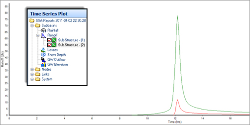
4. On the left side of the screen, expand the Subbasins folder, as shown in Figure 14-38.
5. Click the word Runoff. A plus sign will appear. Click the plus sign to expand the listing.
6. Put a check mark next to both subbasins, as shown in Figure 14-40.
Figure 14-40: The resulting hydrograph from the TR-55 Hydrology analysis
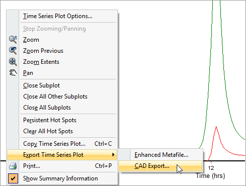
7. Right-click anywhere in the graph area. Select Export Time Series Plot CAD Export, as shown in Figure 14-41.
Figure 14-41: Export To CAD
8. Save the resulting DWG to your desktop as SSA-OUT.dwg.
9. Remain in the SSA project for the next exercise.
A common analysis you will want to examine is the profile plot. On the left side of the SSA window you will see the Profile Plot option. Once the profile plot settings appear, you can graphically select the nodes you wish to include in your output.
In this next exercise, you will examine a profile plot for the pipes in the system.
1. From SSA, continue working in or open the file SSA-Reports.spf. You do not need to have completed the previous exercise to continue—you can download this file from the book’s web page.
2. Click the Perform Analysis button. From the Reports toolbar, select Profile Plot.
3. On the left side of the screen you will see where you can specify Starting Node and Ending Node. You can also specify the link you’d like to plot by clicking on it in the graphic. Click the link Pipe - (1). The pipe will highlight in the plan view.
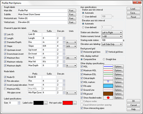
4. Click Plot Options. In the Plot Options dialog, place a check mark next to Maximum Flow, Maximum Velocity, and Maximum Depth. In the Other Display Specifications, place a check mark next to Maximum EGL, Critical Depth, HGL Markers, and Show Flooded Node. Your Profile Plot Options dialog should resemble Figure 14-42. Click OK.
Figure 14-42: Use the Profile Plot Options dialog to control the display of elements in the graphic.
5. Click Show Plot. Your graphic should resemble Figure 14-43.
Figure 14-43: A sample profile plot

After your break from the world of Civil 3D, it is time to export SSA modified data back to CAD. At first glance, you may be thinking that CAD Export or LandXML may be the way to go. However, those options are not the best way to maintain the integrity of your pipe and structure objects. The best option for getting your edits back into Civil 3D is to use File Export Hydraflow Storm Sewers File.
The following exercise will walk you through the steps needed to get back to Civil 3D:
1. From SSA, open the file SSAtoC3D.spf. You can download this file from this book’s web page.
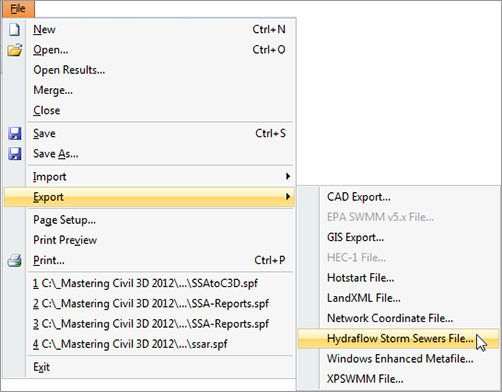
2. Choose File Export Hydraflow Storm Sewers File, as shown in Figure 14-44.
Figure 14-44: Export back to Civil 3D via Hydraflow
3. Save the file as SSAtoC3D.stm on your computer’s desktop.
4. Close SSA.
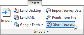
5. In Civil 3D, open the file C3DtoSSA.dwg. From the Import panel, on the Insert tab, select Storm Sewers, as shown in Figure 14-45.
Figure 14-45: Import the file as if it were a storm sewers file
6. Browse to the STM file you exported and click Open. You will get a warning that there is already a pipe network with the same name in the file, as shown in Figure 14-46.
Figure 14-46: Click Update The Existing Pipe Network.
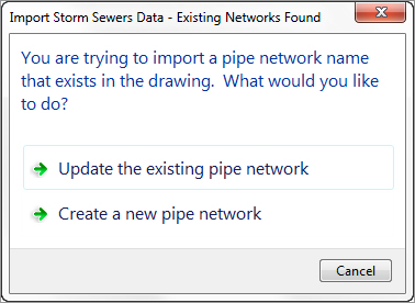
7. Click Update The Existing Pipe Network. After a moment, your pipes and structures should reflect any size or elevation changes that may have occurred in SSA.