
Curves are an important part of surveying and engineering geometry. In truth, curves are no different from AutoCAD arcs. What makes the curve commands different than the basic AutoCAD commands isn’t the resulting arc entity but the inputs used to draw the arc. Civil 3D wants you to provide directions to the arc commands using land surveying terminology rather than with generic Cartesian parameters.
Figure 1-30 shows the Create Curves menu options.
Figure 1-30: Create Curves commands

Standard Curves
When re-creating legal descriptions for roads, easements, and properties, engineers, surveyors, and mappers often encounter a variety of curves. Although standard AutoCAD arc commands could draw these arcs, the AutoCAD arc inputs are designed to be generic to all industries. The following curve commands have been designed to provide an interface that more closely matches land surveying, mapping, and engineering language.
Create Curve Between Two Lines Command
The Create Curve Between Two Lines command is much like the standard AutoCAD Fillet command, except that you aren’t limited to a radius parameter. The command draws a curve that is tangent to two lines of your choosing. This command also trims or extends the original tangents so their endpoints coincide with the curve endpoints. The lines are trimmed or extended to the resulting PC (point of curve, which is the beginning of a curve) and PT (point of tangency, or the end of a curve). You may find this command most useful when you’re creating foundation geometry for road alignments, parcel boundary curves, and similar situations.
The command prompts you to choose the first tangent and then the second tangent. The command line gives the following prompt:
Select entry [Tangent/External/Degree/Chord/Length/Mid-Ordinate/
miN-dist/Radius]<Radius>:
Pressing ↵ at this prompt lets you input your desired radius. As with standard AutoCAD commands, pressing T changes the input parameter to Tangent, pressing C changes the input parameter to Chord, and so on.
As with the Fillet command, your inputs must be geometrically possible. For example, your two lines must allow for a curve of your specifications to be drawn while remaining tangent to both. Figure 1-31 shows two lines with a 25″ radius curve drawn between them. Note that the tangents have been trimmed so their endpoints coincide with the endpoints of the curve. If either line had been too short to meet the endpoint of the curve, then that line would have been extended.
Figure 1-31: Two lines using the Create Curve Between Two Lines command

Create Curve On Two Lines Command
The Create Curve On Two Lines command is identical to the Create Curve Between Two Lines command, except that the Create Curve On Two Lines command leaves the chosen tangents intact. The lines aren’t trimmed or extended to the resulting PC and PT of the curve.
Figure 1-32, for example, shows two lines with a 25″ radius curve drawn on them. The tangents haven’t been trimmed and instead remain exactly as they were drawn before the Create Curve On Two Lines command was executed.
Figure 1-32: The original lines stay the same after you execute the Create Curve On Two Lines command.

Create Curve Through Point Command
The Create Curve Through Point command lets you choose two tangents for your curve followed by a pass-through point. This tool is most useful when you don’t know the radius, length, or other curve parameters but you have two tangents and a target location. It isn’t necessary that the pass-through location be a true point object; it can be any location of your choosing.
This command also trims or extends the original tangents so their endpoints coincide with the curve endpoints. The lines are trimmed or extended to the resulting PC and PT of the curve.
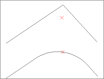
Figure 1-33, for example, shows two lines and a desired pass-through point. Using the Create Curve Through Point command allows you to draw a curve that is tangent to both lines and that passes through the desired point. In this case, the tangents have been trimmed to the PC and PT of the curve.
Figure 1-33: The first image shows two lines with a desired pass-through point. In the second image, the Create Curve Through Point command draws a curve that is tangent to both lines and passes through the chosen point.
Create Multiple Curves Command
The Create Multiple Curves command lets you create several curves that are tangentially connected. The resulting curves have an effect similar to an alignment spiral section. This command can be useful when you are re-creating railway track geometry based on field survey data.
The command prompts you for the two tangents. Then, the command line prompts you as follows:
Enter Number of Curves:
The command allows for up to 10 curves between tangents.
One of your curves must have a flexible length that’s determined on the basis of the lengths, radii, and geometric constraints of the other curves. Curves are counted clockwise, so enter the number of your flexible curve:
Enter Floating Curve #:
Enter the length and radii for all your curves:
Enter curve 1 Radius:
Enter curve 1 Length:
The floating curve number will prompt you for a radius but not a length.
As with all other curve commands, the specified geometry must be possible. If the command can’t find a solution on the basis of your length and radius inputs, it returns no solution (see Figure 1-34).
Figure 1-34: Two curves were specified with the #2 curve designated as the floating curve.

Create Curve From End Of Object Command
The Create Curve From End Of Object command enables you to draw a curve tangent to the end of your chosen line or arc.
The command prompts you to choose an object to serve as the beginning of your curve. You can then specify a radius and an additional parameter (such as Delta or Length) for the curve or the endpoint of the resulting curve chord (see Figure 1-35).
Figure 1-35: A curve, with a 25″ radius and a 30″ length, drawn from the end of a line

Create Reverse Or Compound Curves Command
The Create Reverse Or Compound Curves command allows you to add additional curves to the end of an existing curve. Reverse curves are drawn in the opposite direction (i.e., a curve to the right tangent to a curve to the left) from the original curve to form an S shape. In contrast, compound curves are drawn in the same direction as the original curve (see Figure 1-36). This tool can be useful when you are re-creating a legal description of a road alignment that contains reverse and/or compound curves.
Figure 1-36: A tangent and curve before adding a reverse or compound curve (left); a compound curve drawn from the end of the original curve (right); and a reverse curve drawn from the end of the original curve (bottom)
Re-creating a Deed Using Line and Curve Tools
This exercise will help you apply some of the tools you’ve learned so far to reconstruct the overall parcel that will be used as the sample exercises for the majority of the book.
From Point of Beginning
South 44 degrees 54 minutes 15 seconds West 68.64 feet to a point
North 07 degrees 05 minutes 24 seconds East 217.80 feet to a point
North 72 degrees 12 minutes 10 seconds East 4.23 feet to a point
North 05 degrees 53 minutes 27 seconds East 201.09 feet to a point
South 86 degrees 32 minutes 10 seconds East 121.22 feet to a point
North 03 degrees 25 minutes 51 seconds West 168.78 feet to a point
North 14 degrees 38 minutes 58 seconds East 283.16 feet to a point
North 07 degrees 19 minutes 22 seconds West 79.64 feet to a point
North 07 degrees 04 minutes 00 seconds West 205.45 feet to a point
South 46 degrees 24 minutes 36 seconds West 121.05 feet to a point
South 48 degrees 31 minutes 20 seconds West 414.66 feet to a point
North 49 degrees 29 minutes 56 seconds West 50.80 feet to a point
North 48 degrees 37 minutes 57 seconds East 150.29 feet to a point
North 05 degrees 39 minutes 50 seconds East 497.28 feet to a point
North 84 degrees 20 minutes 01 seconds East 290.33 feet to a point
North 05 degrees 20 minutes 48 seconds West 195.08 feet to a point
North 76 degrees 46 minutes 10 seconds East 701.96 feet to a point
South 23 degrees 42 minutes 48 seconds East 130.68 feet to a point
South 20 degrees 13 minutes 35 seconds East 526.50 feet to a point
South 76 degrees 04 minutes 14 seconds West 379.96 feet to a point
South 13 degrees 22 minutes 41 seconds East 320.08 feet to a point
South 12 degrees 36 minutes 45 seconds East 159.86 feet to a point
South 12 degrees 21 minutes 15 seconds East 274.32 feet to a point
South 61 degrees 15 minutes 09 seconds West 272.81 feet to a point
North 06 degrees 15 minutes 30 seconds West 131.45 feet to a point
South 72 degrees 12 minutes 22 seconds West 301.60 feet to a point
South 06 degrees 58 minutes 04 seconds East 206.04 feet to a point
Returning to Point of Beginning
The resulting enclosure should be: 26.25 acres (more or less)
Follow these steps:
1. Open the Deed Create Start.dwg file, which you can download from this book’s web page at www.sybex.com/masteringcivil3d2012.
2. Turn off Dynamic Input by pressing F12, or by toggling the icon off at the status bar.
3. From the Draw panel on the Home tab, select the Line drop-down and choose the Create Line By Bearing command.
4. At the Select first point: prompt, select any location in the drawing to begin the first line.
5. At the >>Specify quadrant (1-4): prompt, enter 3 to specify the SW quadrant, and then press ↵.
6. At the >>Specify bearing: prompt, enter 44.5415, and press ↵.
7. At the >>Specify distance: prompt, enter 68.64, and press ↵.
8. Repeat steps 4 through 6 for the rest of the courses.
9. Press Esc to exit the Create Line By Bearing command.
10. The finished linework should look like Figure 1-37. There will be an error of closure of 10.0016″. Typically, rounding errors can cause an error in closure. Perhaps reworking the deed holding a different rounding value would improve your results. Consult your office survey expert about how this would be handled in house, and refer to Chapter 2 for more information about traverse adjustment and similar tools.
Figure 1-37: The finished linework

11. Save your drawing. You’ll need it for the next exercise.
Best Fit Entities
Although engineers and surveyors do their best to make their work an exact science, sometimes tools like the Best Fit Entities are required.
Roads in many parts of the world have no defined alignment. They may have been old carriage roads or cart paths from hundreds of years ago that evolved into automobile roads. Surveyors and engineers are often called to help establish official alignments, vertical alignments, and right-of-way lines for such roads on the basis of a best fit of surveyed centerline data.
Other examples for using Best Fit Entities include property lines of agreement, road rehabilitation projects, and other cases where existing survey information must be approximated into “real” engineering geometry (see Figure 1-38).
Figure 1-38: The Create Best Fit Entities menu options

Create Best Fit Line Command
The Create Best Fit Line command under the Best Fit drop-down on the Draw panel takes a series of Civil 3D points, AutoCAD points, entities, or drawing locations and draws a single best-fit line segment from this information. In Figure 1-39, for example, the Create Best Fit Line command draws a best-fit line through a series of points that aren’t quite collinear. Note that the best-fit line will change as more points are picked.
Figure 1-39: A preview line drawn through points that aren’t quite collinear

Once you’ve selected your points, a Panorama window appears with a regression data chart showing information about each point you chose, as shown in Figure 1-40.
Figure 1-40: The Panorama window lets you optimize your best fit.
This interface allows you to optimize your best fit by adding more points, selecting the check box in the Pass Through column to force one of your points on the line, or adjusting the value under the Weight column.
Create Best Fit Arc Command
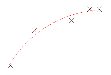
The Create Best Fit Arc command under the Best Fit drop-down works identically to the Create Best Fit Line command, except that the resulting entity is a single arc segment as opposed to a single line segment (see Figure 1-41).
Figure 1-41: A curve created by best fit
Create Best Fit Parabola Command
The Create Parabola command under the Create Best Fit Entities option works in a similar way to the line and arc commands just described. This command is most useful when you have a Triangulated Irregular Network (also known as TIN) sampled or surveyed road information and you’d like to replicate true vertical curves for your design information.
After you select this command, the Parabola By Best Fit dialog appears (see Figure 1-42).
Figure 1-42: The Parabola By Best Fit dialog
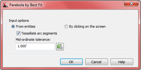
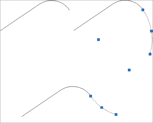
You can select inputs from entities (such as lines, arcs, polylines, or profile objects) or by picking on screen. The command then draws a best-fit parabola on the basis of this information. In Figure 1-43, the shots were represented by AutoCAD points; more points were added by selecting the By Clicking On The Screen option and using the Node osnap to pick each point.
Figure 1-43: The best-fit preview line changes as more points are picked.

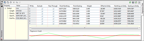
Once you’ve selected your points, a Panorama window appears, showing information about each point you chose. Also note the information in the right pane regarding K-value, curve length, grades, and so forth.
In this interface (shown in Figure 1-44), you can optimize your K-value, length, and other values by adding more points, selecting the check box in the Pass Through column to force one of your points on the line, or adjusting the value under the Weight column.
Figure 1-44: The Panorama window lets you make adjustments to your best-fit parabola.

Attach Multiple Entities
The Attach Multiple Entities command (found on the Home tab and extended Draw panel pull-down) is a combination of the Line From End Of Object command and the Curve From End Of Object command. This command is most useful for reconstructing deeds or road alignments from legal descriptions when each entity is tangent to the previous entity. Using this command saves you time because you don’t have to constantly switch between the Line From End Of Object command and the Curve From End Of Object command (see Figure 1-45).
Figure 1-45: The Attach Multiple Entities command draws a series of lines and arcs so that each segment is tangent to the previous one.

The Curve Calculator
Sometimes you may not have enough information to draw a curve properly. Although many of the curve-creation tools assist you in calculating the curve parameters, you may find an occasion where the deed you’re working with is incomplete.
The Curve Calculator found in the Curves drop-down on the Draw panel helps you calculate a full collection of curve parameters on the basis of your known values and constraints. The units used in the Curve Calculator match the units assigned in your Drawing Settings.
The Curve Calculator can remain open on your screen while you’re working through commands. You can send any value in the Calculator to the command line by clicking the button next to that value (see Figure 1-46).
Figure 1-46: The Curve Calculator

The button at the upper left of the Curve Calculator inherits the arc properties from an existing arc in the drawing, and the drop-down menu in the Degree Of Curve Definition selection field allows you to choose whether to calculate parameters for an arc or a chord definition.
The drop-down menu in the Fixed Property selection field also gives you the choice of fixing your radius or delta value when calculating the values for an arc or a chord, respectively (see Figure 1-47). The parameter chosen as the fixed value is held constant as additional parameters are calculated.
Figure 1-47: The Fixed Property drop-down menu gives you the choice of fixing your radius or delta value.

As explained previously, you can send any value in the Curve Calculator to the command line using the button next to that value. This ability is most useful while you’re active in a curve command and would like to use a certain parameter value to complete the command.
Adding Line and Curve Labels
Although most robust labeling of site geometry is handled using Parcel or Alignment labels, limited line- and curve-annotation tools are available in Civil 3D. The line and curve labels are composed much the same way as other Civil 3D labels, with marked similarities to Parcel and Alignment Segment labels.
Our next exercise leads you through labeling the deed you re-created earlier in this chapter:
1. Continue working in the Deed Create Start.dwg file.
2. Click the Labels button in the Labels & Tables panel on the Annotate tab. The Add Labels dialog appears, as shown in Figure 1-48.
Figure 1-48: The Add Labels dialog, set to Multiple Segment Labels

3. Choose Line And Curve from the Feature drop-down menu.
4. Choose Multiple Segment from the Label Type drop-down menu. The Multiple Segment option places the label at the midpoint of each selected line or arc.
5. Confirm that Line Label Style is set to Bearing Over Distance and that Curve Label Style is set to Distance-Radius And Delta.
6. Click the Add button.
Where Is Delta?
In the Text Component Editor for a curve label, the value that most people would refer to as a delta angle is called the General Segment Total Angle. To insert the Delta symbol in a label, type U+0394 in the Text Editor window on the right side of the Text Component Editor dialog.
7. At the Select Entity: prompt, select each line and arc that you drew in the previous exercise. A label appears on each entity at its midpoint, as shown in Figure 1-49.
Figure 1-49: The labeled linework

8. Save the drawing—you’ll need it for the next exercise.