
Once profile views have been created, things get interesting. The number of modifications to the view itself that can be applied, even before editing the styles, makes profile views one of the most flexible pieces of the Civil 3D package. In this series of exercises, you’ll look at a number of changes that can be applied to any profile view in place.
Profile View Properties
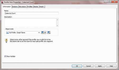
Picking a profile view and selecting Profile View Properties from the Modify View panel yields the dialog shown in Figure 7-63. The properties of a profile include the style applied, station and elevation limits, the number of profiles displayed, and the bands associated with the profile view. If a pipe network is displayed, a tab labeled Pipe Networks will appear.
Figure 7-63: Typical Profile View Properties dialog
Adjusting the Profile View Station Limits
In spite of the wizard, there are often times when a profile view needs to be manually adjusted. For example, the most common change is to limit the length or height (or both) of the alignment that is being shown so it fits on a specific size of paper or viewport. You can make some of these changes during the initial creation of a profile view (as shown in a previous exercise), but you can also make changes after the profile view has been created.
One way to do this is to use the Profile View Properties dialog to make changes to the profile view. The profile view is a Civil 3D object, so it has properties and styles that can be adjusted through this dialog to make the profile view look like you need it to.
1. Open the ProfileViewProperties.dwg file.
2. Zoom to the Cabernet Court profile view.
3. Pick a grid line, and select Profile View Properties from the Modify View panel.
4. On the Stations tab, click the User Specified Range radio button, and set the value of the End station to 7+00, as shown in Figure 7-64.
Figure 7-64: Adjusting the end station values for Cabernet Court

5. Click OK to close the dialog. The profile view will now reflect the updated end station value.
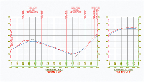
One of the nice things about Civil 3D is that copies of a profile view retain the properties of that view, making a gapped view easy to create manually if they were not created with the wizard.
6. Enter Copy↵ on the command line. Pick the Cabernet Court profile view you just modified.
7. Press F8 on your keyboard to toggle on Ortho mode, and then press ↵.
8. Pick a base point and move the crosshairs to the right. When the crosshairs reach a point where the two profile views do not overlap, pick that as your second point, and press ↵ to end the COPY command.
9. Pick the copy just created and select Profile View Properties from the Modify View panel. The Profile View Properties dialog appears.
10. On the Stations tab, change the stations again. This time, set the Start field to 7+00 and the End field to 9+37.46. The total length of the alignment will now be displayed on the two profile views, with a gap between the two views at station 7+00. Click OK, and your drawing will look like Figure 7-65.
Figure 7-65: A manually created gap between profile views
In addition to creating gapped profile views by changing the profile properties, you can show phase limits by applying a different style to the profile in the second view.
Adjusting the Profile View Elevations
Another common issue is the need to control the height of the profile view. Civil 3D automatically sets the datum and the top elevation of profile views on the basis of the data to be displayed. In most cases this is adequate, but in others, this simply creates a view too large for the space allocated on the sheet or wastes a large amount of that space.
1. Open the ProfileViewProperties.dwg file if you have not already done so.
2. Pan or zoom to the Syrah Way profile view.
3. Select Profile View Properties from the Modify View panel. The Profile View Properties dialog appears.
4. Change to the Elevations tab.
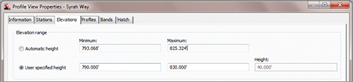
5. In the Elevation Range section, check the User Specified Height radio button and enter the minimum and maximum heights, as shown in Figure 7-66.
Figure 7-66: Modifying the height of the profile view
6. Click OK to close the dialog. The profile view of Syrah Way should reflect the updated elevations, as shown in Figure 7-67.
Figure 7-67: The updated profile view with the heights manually adjusted

The Elevations tab can also be used to split the profile view and create the staggered view that you previously created with the wizard:
1. Pick the Frontenac Drive profile view, right-click a grid line, and select the Profile View Properties option to open the Profile View Properties dialog.
2. Switch to the Elevations tab. In the Elevations Range area, click the User Specified Height radio button.
3. Check the Split Profile View option.
4. Notice that the Height field is now active. Set the height to 36.
5. In the Split Profile View Data section, click the plus (+) icon twice and complete the dialog as shown in Figure 7-68.
Figure 7-68: The Elevations tab

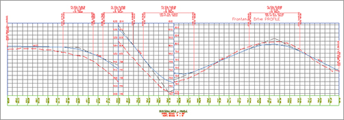
6. Click OK to exit the dialog. The profile view should look like Figure 7-69.
Figure 7-69: A split profile view for the Frontenac Drive alignment
Automatically creating split views is a good starting point, but you’ll often have to tweak them as you’ve done here. The selection of the proper profile view styles is an important part of the Split Profile View process. We’ll look at styles in Chapter 19.
Profile Display Options
Civil 3D allows the creation of literally hundreds of profiles for any given alignment. Doing so makes it easy to evaluate multiple design solutions, but it can also mean that profile views get very crowded. In this exercise, you’ll look at some profile display options that allow the toggling of various profiles within a profile view:
1. Open the ProfileViewProperties1.dwg file.
2. Pick the Cabernet Court profile view, and select Profile View Properties from the Modify View panel. The Profile View Properties dialog appears.
3. Switch to the Profiles tab.
4. Uncheck the Draw option in the EG Surface row and click the Apply button.
5. Drag your dialog out of the way and your profile view should look similar to Figure 7-70.
Figure 7-70: The Cabernet Court profile view with the Draw option toggled off
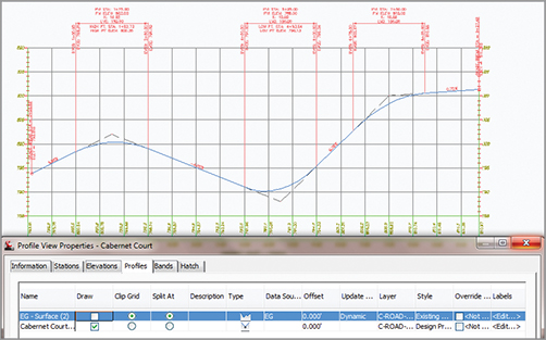
Toggling off the Draw option for the EG surface has created a profile view style in which a profile of the existing ground surface will not be drawn on the profile view.
The sampled profile from the EG surface still exists under the Cabernet Court alignment; it simply isn’t shown in the current profile view. Now that you’ve modified a number of styles, let’s look at another option that is available on the Profile View Properties dialog: bands.
Profile View Bands
Data bands are horizontal elements that display additional information about the profile or alignment that is referenced in a profile view. Bands can be applied to both the top and bottom of a profile view, and there are six different band types:
Profile Data Bands Display information about the selected profile. This information can include simple elements such as elevation, or more complicated information such as the cut-fill between two profiles at the given station.
Vertical Geometry Bands Create an iconic view of the elements making up a profile. Typically used in reference to a design profile, vertical data bands make it easy for a designer to see where vertical curves are located along the alignment.
Horizontal Geometry bands Create a simplified view of the horizontal alignment elements, giving the designer or reviewer information about line, curve, and spiral segments and their relative location to the profile data being displayed.
Superelevation Bands Display the various options for Superelevation values at the critical points along the alignment.
Sectional Data Bands Can display information about the sample line locations, the distance between them, and other sectional-related information.
Pipe Data Bands Can show specific information about each pipe or structure being shown in the profile view.
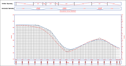
In this exercise, you’ll add bands to give feedback on the EG and layout profiles, as well as horizontal and vertical geometry:
1. Open the ProfileViewBands.dwg file.
2. Zoom out and down to pick the Frontenac Drive profile view, and select Profile View Properties from the Modify View panel. The Profile View Properties dialog appears.
3. Click the Bands tab, as shown in Figure 7-71.
Figure 7-71: The Bands tab of the Profile View Properties dialog
4. Verify that the Band Type drop-down is set to Profile Data and set the Select Band Style drop-down to Elevations And Stations. Click the Add button to display the Geometry Points To Label In Band dialog shown in Figure 7-72.
Figure 7-72: The Geometry Points To Label In Band dialog
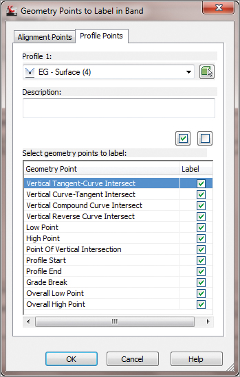
5. Click OK to close the dialog and return to the Profile View Properties dialog. The Profile Data band should now be listed in the middle of the dialog.
6. Set the Location drop-down to Top Of Profile View.
7. Change the Band Type drop-down to the Horizontal Geometry option and choose the Geometry option from the Select Band Style drop-down. Click Add. The Horizontal Geometry band will now be added to the table in the List Of Bands section.
8. Change the Band Type drop-down to Vertical Geometry. Do not change the Select Band Style field from its current selection (Geometry). Click Add. The Vertical Geometry band will also be added to the table in the List Of Bands section.
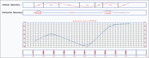
9. Click OK to exit the dialog. Your profile view should look like Figure 7-73.
Figure 7-73: Applying bands to a profile view
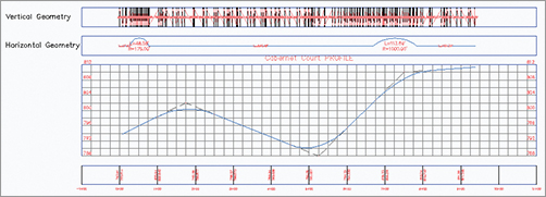
However, there are obviously problems with the bands. The Vertical Geometry band is a mess and is located above the title of the profile view, whereas the Horizontal Geometry band actually overwrites the title. In addition, the elevation information has two numbers with different rounding applied. In this exercise, you’ll fix those issues:
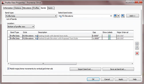
1. Pick the Cabernet Court profile view, and then select Profile View Properties from the Modify View panel. The Profile View Properties dialog appears.
2. Switch to the Bands tab.
3. Verify that the Location drop-down in the List Of Bands section is set to Bottom Of Profile View.
4. Verify that the “Match major/minor increments to vertical grid intervals” option at the bottom of the screen is selected. Checking this option ensures that the major/minor intervals of the profile data band match the major/minor profile view style’s major/minor grid spacing.
5. The Profile Data band is the only band currently listed in the table in the List Of Bands section. Scroll right in the Profile Data row and notice the two columns labeled Profile 1 and Profile 2. Change the value of Profile 2 to Cabernet Court FG, as shown in Figure 7-74.
Figure 7-74: Setting the profile view bands to reference the Cabernet Court FG profile
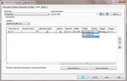
6. Change the Location drop-down to Top Of Profile View.
7. The Horizontal Geometry and the Vertical Geometry bands are now listed in the table as well. Scroll to the right again, and set the value of Profile 1 in the Vertical Geometry band to Cabernet Court FG.
8. Scroll back to the left and set the Gap value for the Horizontal Geometry band to 1.5″. This value controls the distance from one band to the next or to the edge of the profile view itself.
9. Click OK to close the dialog. Your profile view should now look like Figure 7-75.
Figure 7-75: Completed profile view with the Bands set appropriately
Bands use the Profile 1 and Profile 2 designation as part of their style construction. By changing the profile referenced as Profile 1 or 2, you change the values that are calculated and displayed (e.g., existing versus proposed elevations). These bands are just more items that are driven by styles, which you will learn more about in Chapter 19.
Profile View Hatch
Many times it is necessary to shade cut/fill areas in a profile view. The settings on the Hatch tab are used to specify upper and lower cut/fill boundary limits for associated profiles (see Figure 7-76). Shape styles from the General Multipurpose Styles collection found on the Settings tab of Toolspace can also be selected here. These settings include the following:
Figure 7-76: Shape style selection on the Hatch tab of the Profile View Properties dialog

Cut Area Click this button to add hatching to a profile view in areas of the cut.
Fill Area Click this button to add hatching to a profile view in areas of the fill.
Multiple Boundaries Click this button to add hatching to a profile view in areas of a cut/fill where the area must be averaged between two existing profiles (for example, finished ground at the centerline vs. the left and right top of a curb).
From Criteria Click this button to import Quantity Takeoff Criteria.
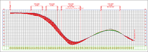
Figure 7-77 shows a cut and fill hatched profile.
Figure 7-77: The Frontenac Drive Profile shown with cut and fill shading
Mastering Profiles and Profile Views
One of the most difficult concepts to master in AutoCAD Civil 3D is the notion of which settings control which display property. Although the following two rules may sound overly simplistic, they are easily forgotten in times of frustration:
- Every object has a label and a style.
- Every label has a style.
Furthermore, if you can remember that there is a distinct difference between a profile object and a profile view object you place it in, you’ll be well on your way to mastering profiles and profile views. When in doubt, select an object, right-click, and pay attention to the Civil 3D commands available.
Profile View Style Selection
Selection of a profile view style is straightforward, but because of the large number of settings in play with a profile view style, the changes can be dramatic. In the following quick exercise, you’ll change the style and see how much a profile view can change in appearance:
1. Open the ProfileViewsModify.dwg file. Remember that all files can be downloaded from www.sybex.com/go/masteringcivil3d2012.
2. Pick a grid line in the Syrah Way profile view and right-click. Notice the available commands.
3. Select the Profile View Properties option. The Profile View Properties dialog opens.
4. On the Information tab, change Object Style to Major Grids and click OK to arrive at Figure 7-78.
Figure 7-78: The Syrah Way profile view with the Major Grids style applied
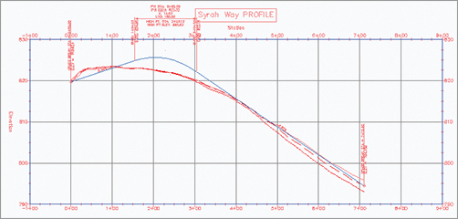
A profile view style includes information such as labeling on the axis, vertical scale factors, grid clipping, and component coloring. Using various styles lets you make changes to the view to meet requirements without changing any of the design information. Changing the style is a straightforward exercise.
Labeling Styles
Now that the profile is labeled, the profile view grid spacing is set, and the titles all look good, it’s time to add some specific callouts and detail information. Civil 3D uses profile view labels and bands for annotating.
View Annotation
Profile view annotations label individual points in a profile view, but they are not tied to a specific profile object. These labels can be used to label a single point or the depth between two points in a profile. We say “depth” because the label recognizes the vertical exaggeration of the profile view and applies the scaling factor to label the correct depth. Profile view labels can be either station elevation or depth labels. In this exercise, you’ll use both:
1. Open the ProfileViewLabels.dwg file.
2. Zoom in on the Syrah Way profile view.
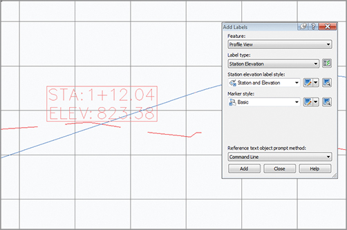
3. Switch to the Annotate tab and select Add Labels from the Labels & Tables panel. The Add Labels dialog opens.
4. In the Feature drop-down, select Profile View; in the Label Type drop-down, verify that Station Elevation is selected; and in the Station Elevation Label Style drop-down, make sure that Station And Elevation is selected.
5. Click the Add button.
6. Click a grid line in the Syrah Way profile view. Zoom in on the right side so that you can see the point where the EG and layout profiles cross over.
7. Pick this profile crossover point visually, and then pick the same point to set the elevation and press ↵. Your label should look like Figure 7-79.
Figure 7-79: An elevation label for a profile station
8. In the Add Labels dialog, change both Label Type and Depth Label Style to the Depth option. Click the Add button.
9. Click a grid line on the Syrah Way profile view.
10. Pick a point along the layout profile and then pick a point along the EG profile and press ↵. The depth between the two profiles will be measured, as shown in Figure 7-80.
Figure 7-80: A depth label applied to the Syrah Way profile view

11. Close the Add Labels dialog.
Why Don’t Snaps Work?
There’s no good answer to this question. For a number of releases now, users have been asking for the ability to simply snap to the intersection of two profiles. We mention this because you’ll try to snap and wonder if you’ve lost your mind. You haven’t—it just doesn’t work. Maybe next year? If you are after a solution (it’s not elegant), you can draw lines on top of the profile.
Depth labels can be handy in earthworks situations where cut and fill become critical, and individual spot labels are important to understanding points of interest, but most design documentation is accomplished with labels placed along the profile view axes in the form of data bands. The next section describes these band sets.
Band Sets
Band sets are simply collections of bands, much like the profile label sets or alignment label sets. In this exercise, you’ll save a band set, and then apply it to a second profile view:
1. Open the ProfileViewBandSets.dwg file.
2. Pick the Syrah Way profile view, and select Profile View Properties from the Modify View panel. The Profile View Properties dialog opens.
3. Switch to the Bands tab.
4. Click the Save As Band Set button to display the Band Set dialog in Figure 7-81.
Figure 7-81: The Information tab for the Band Set dialog

5. In the Name field, enter Elev Station and Horiz Vert Geometry.
6. Click OK to close the Band Set dialog.
7. In the Profiles tab, click the Clip Grid radio button next to Frontenac Drive FG.
8. Click OK to close the Profile View Properties dialog.
9. Pick the Frontenac Drive profile view, and select Profile View Properties from the Modify View panel.
10. Switch to the Bands tab.
11. Click the Import Band Set button, and the Band Set dialog opens.
12. Select the Elev Station and Horiz Vert Geometry option from the drop-down list and click OK.
13. Select Top Of Profile View from the Location drop-down list.
14. Scroll over on the Vertical Geometry and set Profile1 to Frontenac Drive FG.
15. Click OK to exit the Profile View Properties dialog.
16. From the Home tab and Modify panel, select Match Properties. You can also type MA↵.
17. At the Select source object: prompt, select the profile grid on Syrah Way.
18. At the Select destination object(s) or [Settings]: prompt, select the profile grid on Frontenac Drive.
19. The grid for Frontenac Drive now matches the Syrah Way profile. Your profile view should look like Figure 7-82.
Figure 7-82: Completed profile view after importing the band set and matching properties
Your Frontenac Drive profile view now looks like the Syrah Way profile view. Band sets allow you to create uniform labeling and callout information across a variety of profile views. By using a band set, you can apply myriad settings and styles that you’ve assigned to a single profile view to a number of profile views. The simplicity of enforcing standard profile view labels and styles makes using profiles and profile views simpler than ever.
Bring Out the Band
Once design speeds have been assigned to an alignment, and superelevation has been calculated, you’ll find the Superelevation View command on the Modify panel of the Alignment context menu. Although not the focus of this chapter, superelevation views behave much like profile views, and you can access their properties via the right-click menu after selecting a view.