
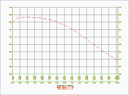
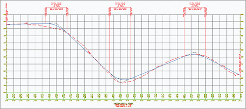
The whole point of a three-dimensional model is to include the elevation element that’s been missing for years. But to get there, designers and engineers still depend on a flat 2D representation of the vertical dimension as shown in a profile view (see Figure 7-1).
Figure 7-1: A typical profile view of the surface elevation along an alignment
A profile is nothing more than a series of data pairs in a station, elevation format. There are basic curve and tangent components, but these are purely the mathematical basis for the paired data sets. In Civil 3D, you can generate profile information in one of the following three ways:
- Sampling from a surface involves taking vertical information from a surface object every time the sampled alignment crosses a TIN line of the surface.
- Using a layout to create a profile allows you to input design information, setting critical station and elevation points, calculating curves to connect linear segments, and typically working within requirements laid out by a reviewing agency.
- Creating from a file lets you point to a specially formatted text file to pull in the station and elevation pairs. Doing so can be helpful in dealing with other analysis packages or spreadsheet tabular data.
This section looks at all three methods of creating profiles.
Surface Sampling
Working with surface information is the most elemental method of creating a profile. This information can represent a simple existing or proposed surface, a river flood elevation, or any number of other surface-derived data sets. Within Civil 3D, surfaces can also be sampled at offsets, as you’ll see in the next series of exercises. Follow these steps:
1. Open the ProfileSampling.dwg file shown in Figure 7-2. (Remember, all data files can be downloaded from this book’s web page at www.sybex.com/go/masteringcivil3d2012.)
Figure 7-2: The drawing you’ll use for this exercise

2. Select Create Surface Profile from the Profile drop-down on the Create Design panel to open the Create Profile From Surface dialog, as shown in Figure 7-3.
Figure 7-3: The Create Profile From Surface dialog
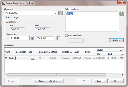
This dialog has a number of important features, so take a moment to see how it breaks down:
- The upper-left quadrant is dedicated to information about the alignment. You can select the alignment from a drop-down list, or you can click the Pick On Screen icon. The Station Range area is automatically set to run from the beginning to the end of the alignment, but you can control it manually by entering the station ranges in the To Sample text boxes or by using the station pick icons.
- The upper-right quadrant controls the selection of the surface and the offsets. You can select a surface from the list, or you can click the Pick On Screen icon. Beneath the Select Surfaces list box is a Sample Offsets check box. The offsets aren’t applied in the left and right direction uniformly. You must enter a negative value to sample to the left of the alignment or a positive value to sample to the right. In all cases, the profile isn’t generated until you click the Add button. You can add multiple offsets here—for example: –50, 25,–10,–5,0,5,10,25,50
- The Profile List box displays all profiles associated with the alignment currently selected in the Alignment drop-down menu. This area is generally static (it won’t change), but you can modify the Update Mode, Layer, and Style columns by clicking the appropriate cells in this table. You can stretch and rearrange the columns to customize the view.
3. Select the Syrah Way option from the Alignment drop-down menu if it isn’t already selected.
4. In the Select Surfaces list area, select EG.
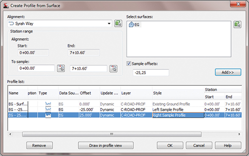
5. Select the Sample Offsets check box to make the entry box active, and enter –25,25.
6. Click Add again. The dialog should look like Figure 7-4.
Figure 7-4: The Create Profile From Surface dialog showing the profiles sampled on surface EG

7. In the Profile List area, select the cell in the Style column that corresponds to the –25.000′ value in the Offset column (see Figure 7-4) to activate the Pick Profile Style dialog.
8. Select the Left Sample Profile option, and click OK. The style changes from Existing Ground Profile to Left Sample Profile in the table.
9. Select the cell in the Style column that corresponds to the 25.000’ value in the Offset column.
10. Select the Right Sample Profile option, and click OK. The dialog should look like Figure 7-5.
Figure 7-5: The Create Profile From Surface dialog with styles assigned on the basis of the Offset value
11. Click OK to dismiss this dialog.
12. The Events tab in Panorama appears, telling you that you’ve sampled data or if an error in the sampling needs to be fixed. Click the green check mark or the X to dismiss Panorama.
Profiles are dependent on the alignment they’re derived from, so they’re stored as profile branches under their parent alignment on the Prospector tab, as shown in Figure 7-6.
Figure 7-6: Alignment profiles on the Prospector tab

Aren’t You Going to Draw the Profile View?
Under normal conditions, you would click the Draw In Profile View button to go through the process of creating the grid, labels, and other components that are part of a completed profile view. You’ll skip that step for now because you’re focusing on the profiles themselves.
By maintaining the profiles under the alignments, it becomes simpler to review what has been sampled and modified for each alignment. Note that the profiles are dynamic and continuously update, as you’ll see in this exercise:
1. Open the DynamicProfiles.dwg file.
2. On the Viewport Controls located at the upper left of the drawing screen, select Viewport Configurations Two: Horizontal.
3. Click in the top viewport to activate it.
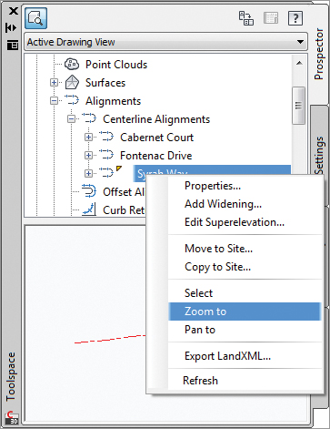
4. On the Prospector tab, expand the Alignments branch to view the alignment types, expand the Centerline Alignments branch, and right-click Syrah Way. Select the Zoom To option, as shown in Figure 7-7.
Figure 7-7: The Zoom To option on Syrah Way
5. Click in the bottom viewport to activate it.
6. Expand the Alignments Centerline Alignments Syrah Way Profile Views branches.
7. Right-click Syrah Way, and select Zoom To. Your screen should now look similar to Figure 7-8.
Figure 7-8: Splitting the screen for plan and profile editing

8. Click in the top viewport.
9. Zoom out so you can see more of the plan view.
10. Pick the alignment to activate the grips, and stretch a beginning grip to lengthen the alignment, as shown in Figure 7-9.
Figure 7-9: Grip-editing the alignment

11. Click to complete the edit. The alignment profile (the red lines) automatically adjusts to reflect the change in the starting point of the alignment. Note that the offset profiles move dynamically as well.
By maintaining the relationships between the alignment, the surface, the sampled information, and the offsets, Civil 3D creates a much more dynamic feedback system for designers. This system can be useful when you’re analyzing a situation with a number of possible solutions, where the surface information will be a deciding factor in the final location of the alignment. Once you’ve selected a location, you can use this profile view to create a vertical design, as you’ll see in the next section.
Left to Right and Right to Left?
You may have noticed that the alignment for Syrah Way is drawn right to left but the profile shows it left to right. It is often desirable to have the plan and profile go in the same direction. There are a number of things you can do to fix this:
- Rotate the plan view 180 degrees. If you have your labeling all set to be plan-readable, it will follow along nicely.
- Consider changing the profile to read from right to left:
- Right-click the profile view (grid) and select Profile View Properties.
- On the Information tab, change Object Style to Full Profile - RIGHT TO LEFT.
- Click OK.
To learn more about styles, refer to Chapter 19, “Styles.”
Layout Profiles
Working with sampled surface information is dynamic, and the improvement over previous generations of Autodesk Civil design software is profound. Moving into the design stage, you’ll see how these improvements continue as you look at the nature of creating design profiles. By working with layout profiles as a collection of components that understand their relationships with each other as opposed to independent finite elements, you can continue to use the program as a design tool instead of just a drafting tool.
You can create layout profiles in two basic ways:
- PVI-based layouts are the most common, using tangents between points of vertical intersection (PVIs) and then applying curve parameters to connect them. PVI-based editing allows editing in a more conventional tabular format.
- Entity-based layouts operate like horizontal alignments in the use of free, floating, and fixed entities. The PVI points are derived from pass-through points and other parameters that are used to create the entities. Entity-based editing allows for the selection of individual entities and editing in an individual component dialog.
You’ll work with both methods in the next series of exercises to illustrate a variety of creation and editing techniques. First, you’ll focus on the initial layout, and then you’ll edit the various layouts.
Layout by PVI
PVI layout is the most common methodology in transportation design. Using long tangents that connect PVIs by derived parabolic curves is a method most engineers are familiar with, and it’s the method you’ll use in the first exercise:
1. Open the LayoutProfiles-PVI.dwg file.
2. On the Home tab’s Create Design panel, select Profiles Profile Creation Tools.
3. Pick the Syrah Way profile view by clicking one of the grid lines. The Create Profile dialog appears, as shown in Figure 7-10.
Figure 7-10: The Create Profile dialog

4. Make the changes as shown in Figure 7-10. Click OK. The Profile Layout Tools toolbar appears. Notice that the toolbar is modeless, meaning it stays open even if you do other AutoCAD operations such as Pan or Zoom.
At this point, you’re ready to begin laying out your vertical design. Before you do, however, note that this exercise skips two options. The first is the idea of profile label sets. You’ll explore them in a later section of this chapter. The other option is Criteria-Based Design on the Design tab. Criteria-based design operates in profiles similar to Chapter 6, “Alignments,” in that the software compares the design speed to a selected design table (typically AASHTO 2001 in the North America releases) and sets minimum values for curve K values. This can be helpful when you’re laying out long highway design projects, but most site and subdivision designers have other criteria to design against.
5. On the toolbar, click the arrow by the Draw Tangents tool on the far left.
6. Select the Curve Settings option. The Vertical Curve Settings dialog opens, as shown in Figure 7-11.
Figure 7-11: The Vertical Curve Settings dialog
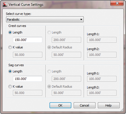
7. The Select Curve Type drop-down menu should be set to Parabolic, and the Length values in both the Crest Curves and Sag Curves areas should be 150.000′, as shown in Figure 7-11. Selecting a Circular or Asymmetric curve type activates the other options in this dialog.
To K or Not to K
You don’t have to choose. Realizing that users need to be able to design using both, Civil 3D 2012 lets you modify your design based on what’s important. You can enter a K value to see the required length, and then enter a nice even length that satisfies the K. The choice is up to you.
8. Click OK to close the Vertical Curve Settings dialog.
9. On the Profile Layout Tools toolbar, click the arrow next to the Draw Tangents Without Curves tool again. This time, select the Draw Tangents With Curves option.
10. Use a Center osnap to pick the center of the circle at far right in the profile view. A jig line, which will be your layout profile, appears. Remember, the profile is reversed so that station 0+00 is lined up with the plan. Therefore, Station 0+00 is on the right of the profile.
11. Continue working your way across the profile view, picking the center of each circle with a Center osnap.
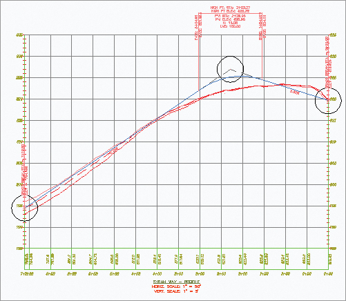
12. Right-click or press ↵ after you select the center of the last circle; your drawing should look like Figure 7-12.
Figure 7-12: A completed layout profile with labels
What Is a Jig?
A jig is a temporary line shown onscreen to help you locate your pick point. Jigs work in a similar way to osnaps in that they give feedback during command use but then disappear when the selection is complete. Civil 3D uses jigs to help you locate information on the screen for alignments, profiles, profile views, and a number of other places where a little feedback goes a long way.
The layout profile is labeled with the Complete Label Set you selected in the Create Profile dialog. As you’d expect, this labeling and the layout profile are dynamic. If you click and then zoom in on this profile line, not the labels or the profile view, you’ll see something like Figure 7-13.
Figure 7-13: The types of grips on a layout profile

The PVI-based layout profiles include the following unique grips:
- The red triangle at the PVI point is the PVI grip. Moving this alters the inbound and outbound tangents, but the curve remains in place with the same design parameters of length and type.
- The triangular grips on either side of the PVI are sliding PVI grips. Selecting and moving either moves the PVI, but movement is limited to along the tangent of the selected grip. The curve length isn’t affected by moving these grips.
- The circular grips near the PVI and at each end of the curve are curve grips. Moving any of these grips makes the curve longer or shorter without adjusting the inbound or outbound tangents or the PVI point.
Although this simple pick-and-go methodology works for preliminary layout, it lacks a certain amount of control typically required for final design. For that, you’ll use another method of creating PVIs:
1. Open the LayoutProfiles-Transparent.dwg file. Make sure the Transparent Commands toolbar (Figure 7-14) is displayed somewhere on your screen.
Figure 7-14: The Transparent Commands toolbar
2. On the Home tab’s Create Design panel, select Profiles Profile Creation Tools.
3. Pick a grid line on the Cabernet Court profile view to display the Create Profile – Draw New dialog.
4. Change the name to Cabernet Court FG and then click OK.
5. On the Profile Layout Tools toolbar, click the drop-down menu by the Draw Tangents Without Curves tool, and select the Draw Tangents With Curves tool, as in the previous exercise. Use a Center osnap to snap to the center of the circle at the left edge of the profile view.
6. On the Transparent Commands toolbar, select the Profile Station Elevation command.
7. Pick a grid line on the profile view. If you move your cursor within the profile grid area, a vertical red line, or jig, appears; it moves up and down and from side to side. Notice the tooltips.
8. Enter 175↵ at the command line for the station value. If you move your cursor within the profile grid area, a horizontal and vertical jig appears (see Figure 7-15), but it can only move vertically along station 175. If you’ve turned on Dynamic Input, the text in the white box shows the elevation along the 175 jig, and the text in the black box shows the horizontal and vertical location of the cursor.
Figure 7-15: A jig appears when you use the Profile Station Elevation transparent command.

9. Enter 802↵ at the command line to set the elevation for the second PVI.
10. Press Esc only once. The Profile Station Elevation command is no longer active, but the Draw Tangents With Curves tool that you previously selected on the Profile Layout Tools toolbar continues to be active.
11. On the Transparent Commands toolbar, select the Profile Grade Station command.
12. Enter –4↵ at the command line for the profile grade.
13. Enter 525↵ for the station value at the command line. Press Esc only once to deactivate the Profile Grade Station command.
14. On the Transparent Commands toolbar, select the Profile Grade Length command.
15. Enter 9.78↵ at the command line for the profile grade.
16. Enter 225↵ for the profile grade length.
17. Press Esc only once to deactivate the Profile Grade Length command and to continue using the Draw Tangent With Curves tool.
18. Use a Center osnap to select the center of the circle along the far-right side of the profile view.
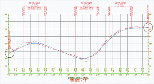
19. Press ↵ to complete the profile. Your profile should look like Figure 7-16.
Figure 7-16: Using the Transparent Commands toolbar to create a layout profile
Using PVIs to define tangents and fitting curves between them is the most common approach to create a layout profile, but you’ll look at an entity-based design in the next section.
Layout by Entity
Working with the concepts of fixed, floating, and free entities as you did in Chapter 6, you’ll lay out a design profile in this exercise:
1. Open the LayoutProfiles-Entity.dwg file.
2. On the Home tab’s Create Design panel, select Profiles Profile Creation Tools.
3. Pick a grid line on the Syrah Way profile view to display the Create Profile dialog.
4. Change the name to Syrah Way FG, click OK, and open the Profile Layout Tools toolbar.
Right to Left
Remember that as we use the Syrah Way profile it has been created from right to left.
5. Click the arrow by the Draw Fixed Tangent By Two Points tool, and select the Fixed Tangent (Two Points).
6. Using a Center osnap, pick the circle at the right edge of the profile view. A rubber-banding line appears.
7. Using a Center osnap, pick the circle located at approximately station 1+50. A tangent is drawn between these two circles.
8. Using a Center osnap, pick the circle located at approximately station 3+00. Another rubber-banding line appears.
9. Using a Center osnap, pick the circle located at the left edge of the profile view. A second tangent is drawn. Right-click to exit the Fixed Tangent (Two Points) command; your drawing should look like Figure 7-17.
Figure 7-17: Layout profile with two tangents drawn
10. Click the arrow next to the Draw Fixed Parabola By Three Points tool on the Profile Layout Tools toolbar.
11. Choose the More Fixed Vertical Curves Fixed Vertical Curve (Entity End, Through Point) option.
12. Pick the right tangent to attach the fixed vertical curve. Remember to pick the tangent line and not the end circle. A rubber-banding line appears.
13. Using a Center osnap, select the circle located at approximately station 3+00.
14. Right-click to exit the Fixed Vertical Curve (Entity End, Through Point) command. Your drawing should look like Figure 7-18.
Figure 7-18: Completed curve from the entity end

With the entity-creation method, grip editing works in a similar way to other layout methods. You’ll look at more editing methods after trying the final creation method.
The Best Fit Profile
You’ve surveyed along a centerline, and you need to closely approximate the tangents and vertical curves as they were originally designed and constructed.
A best fit profile can be created from AutoCAD blocks, AutoCAD 3D polylines, AutoCAD points, COGO points, a surface profile, or feature lines. The most common option is the surface profile. The tool attempts to run a complex algorithm to determine the best fit profile path, including both tangents and vertical curves. However, the only best fit option available for determining vertical curves is the maximum curve radius. The maximum curve radius is a formula rarely used in the design of parabolic curves, the most common curves found in roadway design. Unlike the Best Fit tool for lines and curves as seen in Chapter 1, “The Basics of Civil 3D,” this tool has no options for selecting or deselecting points, making the tool somewhat cumbersome.
The Create Best Fit Profile tool is found on the Profile drop-down on the Create Design panel on the Home tab.
In many cases, the tools you choose to use in a given scenario, as promising as the name may sound, may actually prove to be more of a hindrance than they are helpful. The Best Fit Profile tool may be one of these cases. The tool attempts to perform an analysis on all the sampled existing ground profile points in a profile view, the options are limited, and in the end, you may find a good pair of eyes and graphical analysis using other profile creation tools to be less time consuming. It’s important to understand all the tools at your disposal, but you are not required to use each one in a production environment. If results don’t meet your needs and you’ve spent considerable time with a single tool, find another tool, or tools, that accomplish the same task. Remember, at the end of the day, you still have sheets to cut and plans to get out the door. You’re limited only by your selection of tools and your creativity.
Creating a Profile from a File
Working with profile information in Civil 3D is nice, but it’s not the only place where you can create or manipulate this sort of information. Many programs or analysis packages generate profile information. One common case is the plotting of a hydraulic grade line against a stormwater network profile of the pipes. When information comes from outside the Civil 3D program, it’s often output in myriad formats. If you convert this format to the required format for Civil 3D, the profile information can be input directly.
Civil 3D has a specific format. Each line is a PVI definition (station and elevation). Curve information is an optional third bit of data on any line. Here’s one example:
0 550.76
127.5 552.24
200.8 554 100
256.8 557.78 50
310.75 561
In this example, the third and fourth lines include the curve length as the optional third piece of information. The only inconvenience of using this input method is that the information in Civil 3D doesn’t directly reference the text file. Once the profile data is imported, no dynamic relationship exists with the text file.
In this exercise, you’ll import a small text file to see how the function works:
1. Open the ProfilefromFile.dwg file.
2. On the Home tab’s Create Design panel, select Profiles Create Profile From File.
3. Select the ProfileFromFile.txt file, and click Open. The Create Profile dialog appears.
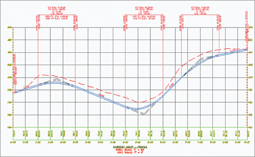
4. In the dialog, choose Frontenac Drive for the Name, Design Profile from the Profile Style, and Complete Label Set from the Profile Label Set drop-down menu.
5. Click OK. Your drawing should look like Figure 7-19.
Figure 7-19: A completed profile created from a file
Now that you’ve tried the three main ways of creating profile information, you’ll edit a profile in the next section.
Profile Layout Tools
Although we have touched on many of the available tools in the Profile Layout Tools palette, there are still many that we have not.
Draw Tangents Profile layout point to point. No curves.
Draw Tangents With Curves Profile layout point to point with curve type and length determined from Curve Settings.
Curve Settings Sets the type of curve (Parabolic, Circular, Asymmetric), K factor, and length.
Insert PVI Inserts a PVI at the specified location.
Delete PVI Deletes a PVI at the specified location.
Move PVI Moves a PVI at the specified location.
Convert AutoCAD Line And Spline Takes a singular line/spline and converts it into a profile object.
Insert PVI Tabular Allows you to enter PVI station and elevation information in a table-like dialog.
Raise/Lower PVI Allows you to raise or lower a profile at a specified distance and either the entire profile or a specified station range.
Copy Profile Copies a profile.
PVI or Entity-Based Display profile layout tools based on either PVI or Entity.
Select PVI Opens the Profile Layout Parameters dialog for the selected PVI.
Delete Entity Deletes a profile subobject curve and turns it into tangents.
Profile Layout Parameters Opens the Profile Layout Parameters dialog.
Profile Grid Box Opens the Entities Panorama showing all segments of the profile.
Editing Profiles
The methods just reviewed let you quickly create profiles. You saw how sampled profiles reflect changes in the parent alignment and how some grips are available on layout profiles, and you also imported a text file that could easily be modified. In all these cases, the editing methods left something to be desired, from either a precision or a dynamic relationship viewpoint.
This section looks at profile editing methods. The most basic is a more precise grip-editing methodology, which you’ll learn about first. Then you’ll see how to modify the PVI-based layout profile, how to change out the components that make up a layout profile, and how to use editing functions that don’t fit into a nice category.
Grip Profile Editing
Once a layout is in place, sometimes a simple grip edit will suffice. But for precision editing, you can use a combination of the grips and the tools on the Transparent Commands toolbar, as in this short exercise:
1. Open the GripEditingProfiles.dwg file.
2. Zoom in, and pick the layout profile for Frontenac Drive (the blue line) to activate its grips.
3. Pick the triangular grip pointing upward on the left vertical curve that is around Sta. 8+00 to begin a grip stretch of the PVI, as shown in Figure 7-20.
Figure 7-20: Grip-editing a PVI

4. On the Transparent Commands toolbar, select the Profile Station Elevation command.
5. Pick a grid line on the profile view.
6. Enter 801↵ at the command line to set the profile station.
7. Enter 781↵ to set the profile elevation.
8. Press Esc to deselect the layout profile object you selected in step 2, and regenerate your view to complete the changes, as shown in Figure 7-21.
Figure 7-21: Completed grip edit using the transparent commands for precision

The grips can go from quick-and-dirty editing tools to precise editing tools when you use them in conjunction with the transparent commands in the profile view. They lack the ability to precisely control a curve length, though, so you’ll look at editing a curve next.
Parameter and Panorama Profile Editing
Beyond the simple grip edits, but before changing out the components of a typical profile, you can modify the values that drive an individual component. In this exercise, you’ll use the Profile Layout Parameter dialog and the Panorama palette set to modify the curve properties on your design profile:
1. Open the ParameterEditingProfiles.dwg file.
2. Pick the layout profile for Frontenac Drive (the blue line) to activate its grips.
3. Select Geometry Editor from the Modify Profile panel.
4. On the Profile Layout Tools toolbar, click the Profile Layout Parameters tool to open the Profile Layout Parameters dialog.
5. Click the Select PVI tool, and zoom in to click near the PVI near station 13+25 to populate the Profile Layout Parameters dialog (Figure 7-22).
Figure 7-22: The Profile Layout Parameters dialog
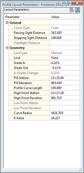
Values that can be edited are in black; the rest are mathematically derived and can be of some design value but can’t be directly modified. The two buttons at the top of the dialog adjust how much information is displayed.
6. Change the Profile Curve Length in the Profile Layout Parameters dialog to 250.000′ (see Figure 7-23).
Figure 7-23: Direct editing of the curve layout parameters

7. Close the Profile Layout Parameters dialog by clicking the red X in the upper-right corner. Then, press the Esc key to deactivate the Select PVI tool.
8. On the Profile Layout Tools toolbar, click the Profile Grid View tool to activate the Profile Entities tab in Panorama. Panorama allows you to view all the profile components at once, in a compact form.
9. Scroll right in Panorama until you see the Profile Curve Length column.
10. Double-click in the cell for the Entity 2 value in the Profile Curve Length column (see Figure 7-24), and change the value from 150.000′ to 250.000’.
Figure 7-24: Direct editing of the curve length in Panorama

11. Close the Profile Layout Tools toolbar, and zoom out to review your edits. Your complete profile should now look like Figure 7-25.
Figure 7-25: The completed editing of the curve length in the layout profile

You can use these tools to modify the PVI points or tangent parameters, but they won’t let you add or remove an entire component. You’ll do that in the next section.
PVIs in Lockdown
You can lock a PVI at a specific station and elevation in the Profile Layout Parameters dialog. PVIs that are locked cannot be moved with edits to adjacent entities. However, it’s important to note that a PVI can be unlocked with editing grips.
Component-Level Editing
In addition to editing basic parameters and locations, sometimes you have to add or remove entire components. In this exercise, you’ll add a PVI, remove a curve from an area that no longer requires one, and insert a new curve into the layout profile:
1. Open the ComponentEditingProfiles.dwg file.
2. Select the layout profile to activate its grips.
3. Select Geometry Editor from the Modify Profile panel.
4. On the Profile Layout Tools toolbar, click the Insert PVI tool.
5. Pick a point near the 5+50 station, with an approximate elevation of 815. The position of the tangents on either side of this new PVI is affected, and the profile is adjusted accordingly. The vertical curves that were in place are also modified to accommodate this new geometry.
6. On the Profile Layout Tools toolbar, click the Delete Entity tool. Notice the grips disappear and the labels update.
7. Zoom in, and pick the curve entity near station 3+50 to delete it. Then, right-click to update the display.
8. On the Profile Layout Tools toolbar, click the arrow by the Draw Fixed Vertical Curve By Three Points tool. Select the More Free Vertical Curves Free Vertical Parabola (PVI Based) option.
9. Pick near the PVI you just inserted (near the 5+50 station in step 5) to add a curve.
10. Enter 150↵ at the command line to set the curve length.
11. Repeat steps 8–10, but use the PVI near 3+50.
12. Right-click to exit the command and update the profile display.
13. Close the Profile Layout Tools toolbar. Your drawing should look similar to Figure 7-26.
Figure 7-26: The completed editing of the curve using component-level editing

Editing profiles using any of these methods gives you precise control over the creation and layout of your vertical design. In addition to these tools, some of the tools on the Profile Layout Tools toolbar are worth investigating and somewhat defy these categories. You’ll look at them next.
Other Profile Edits
Some handy tools exist on the Profile Layout Tools toolbar for performing specific actions. These tools aren’t normally used during the preliminary design stage, but they come into play as you’re working to create a final design for grading or corridor design. They include raising or lowering a whole layout in one shot, as well as copying profiles. Try this exercise:
1. Open the OtherProfileEdits.dwg file.
2. Zoom to the Cabernet Court Profile if it not already showing.
3. Pick the Cabernet Court FG profile to activate its grips. It is the blue line.
4. Select Geometry Editor from the Modify Profile panel. The Profile Layout Tools toolbar appears.
5. Click the Raise/Lower PVIs tool. The Raise/Lower PVI Elevation dialog shown here appears:
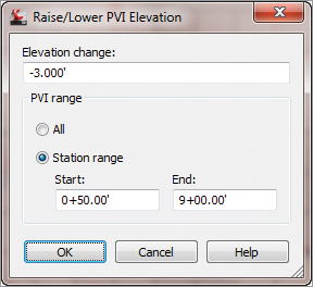
6. Set Elevation Change to –3.000′. Click the Station Range radio button, and set the Start value to 0+50′ and the End value to 9+00.00’. Click OK.
7. Click the Copy Profile tool to display the Copy Profile Data dialog.

8. Click OK to create a new layout profile directly on top of Layout 1. Note that after picking the newly created layout profile, the Profile Layout Tools toolbar now references this newly created Layout (2) profile.
9. Use the Raise/Lower tool to drop Layout (2) by 0.5’ to simulate an edge-of-pavement design. Your drawing should look similar to this:
Using the layout and editing tools in these sections, you should be able to design and draw a combination of profile information presented to you as a Civil 3D user.
Matching Profile Elevations
Up to now, you have learned how to use some of the available tools for modifying profiles. Now let’s try to tie it all together in our subdivision.
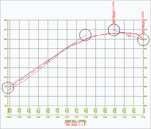
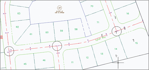
If you take a look at Figure 7-27, you will see that Syrah Way actually has three road intersections, which are circled: two for Frontenac Drive and one for Cabernet Court. We need to know the elevation for the intersecting point between these intersections. First, let’s look at the station where the intersections occur:
Figure 7-27: Syrah Way and the intersecting roads
1. Open the RoadsMatchProfiles.dwg file.
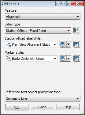
2. From the Annotate tab and Labels & Tables panel, select Add Labels. The Add Labels dialog opens.
3. Change the feature type to Alignment, label type to Station Offset - Fixed Point, and station offset label style type to Plan View Alignment Station Check, as shown in Figure 7-28. Click Add.
Figure 7-28: Syrah Way and the intersecting roads
4. At the Select alignment: prompt, click on the alignment for Syrah Way. This sets Syrah Way as the main alignment that will be used.
5. At the Select point: prompt, use an endpoint osnap and use Frontenac Drive Station 0+00 as the point.
6. At the Select alignment for label style component Reference Alignment: prompt, select anywhere on Frontenac Drive.
7. Right-click to end the command.
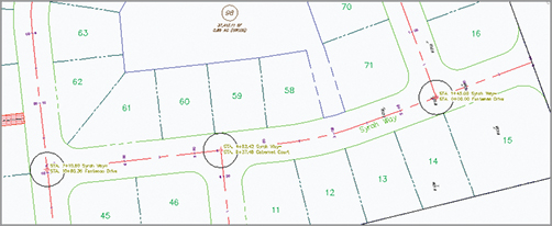
A label showing the station of Syrah Way and Frontenac Drive intersection appears. You will need this information for the next step, but first rerun the Plan View Alignment Station Check label for the next two intersections. Your drawing should look similar to Figure 7-29.
Figure 7-29: Syrah Way and the intersecting roads
Now that you have established the stations at which the intersections occur, let’s put the intersecting stations into practice on the profiles:
1. Continuing with the same drawing, set your viewports to Two: Horizontal so you can see the Syrah Way plan view on top and the profile view on the bottom.
2. From the Annotate tab and Labels & Tables panel, select Add Labels. The Add Labels dialog opens.
3. Change the feature type to Profile View, label type to Station Elevation, and station elevation label style to Station And Elevation Reference Alignment RIGHT; then click Add.
4. At the Select a profile view: prompt, select Syrah Way.
5. At the Specify station: prompt, refer to the plan view and type 145 as the first label indicates. Remember, the Syrah Way profile goes from right to left.
6. At the Specify elevation: prompt, pick anywhere on your drawing. For this case, the location is not important as we will address that in a bit.
7. You are now prompted to select alignment for the label style component Alignment Ref:. Select the top viewport and choose Frontenac Drive.
8. Press Esc. Your label should look like Figure 7-30.
Figure 7-30: The alignment intersection label
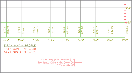
You can see that everything is populated except the elevation, which is the most important piece of information needed.
9. Select the newly created label. In the Properties General area, click in the Profile1 Object. Click the Selector icon.
10. At the Select an object <or press Enter key to select from list>: prompt, press ↵, select the Syrah Way FG object, and click OK.
The Elevation portion of the label is now populated with the elevation, which is 824.50. This is the starting elevation of Frontenac Drive in order to make both roads meet.
Repeat steps 1–10 for the other two elevation labels. If you wish to move the label, we recommend that you turn Ortho mode on so you keep the same station. Your profile should look like Figure 7-31.
Figure 7-31: The Alignment Intersection label updated

Now you have all the pieces you need. Modify the profiles using any of the previously mentioned methods so that the beginning of Frontenac Drive matches elevation 824.50 and the end of Cabernet Court matches elevation of 811.36. Further, you can lock these elevations since they are critical by selecting the lock icon in the Profile Entities Panorama.
Profile Display
No matter how profiles are created, they need to be shown and labeled to make the information more understandable. In this section, you’ll learn about options for the profile labels.
Styles: Where to Look
The exercises in this chapter have many different styles created to show variety. You’ll learn more about styles in Chapter 19, “Styles.” It’s okay to take a peek ahead once in a while.
Profile Labels
It’s important to remember that the profile and the profile view aren’t the same thing. The labels discussed in this section are those that relate directly to the profile. This usually means station-based labels, individual tangent and curve labels, or grade breaks.
Applying Labels
As with alignments, you apply labels as a group of objects separate from the profile. In this exercise, you’ll learn how to add labels along a profile object:
1. Open the ApplyingProfileLabels.dwg file.
2. Pick the layout profile (the blue line) to activate the profile object.
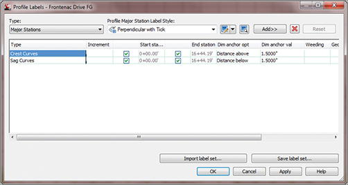
3. Select Edit Profile Labels from the Labels panel to display the Profile Labels dialog (see Figure 7-32).
Figure 7-32: An empty Profile Labels dialog
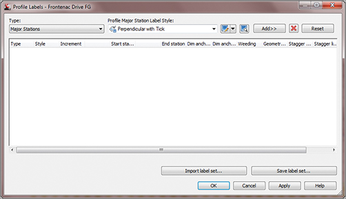
Selecting the type of label from the Type drop-down menu changes the Style drop-down menu to include styles that are available for that label type. Next to the Style drop-down menu are the usual Style Edit/Copy button and a preview button. Once you’ve selected a style from the Style drop-down menu, clicking the Add button places it on the profile. The middle portion of this dialog displays information about the labels that are being applied to the profile selected; you’ll look at that in a moment.
4. Choose the Major Stations option from the Type drop-down menu. The name of the second drop-down menu changes to Profile Major Station Label Style to reflect this option. Verify that Perpendicular With Tick is selected in this menu.
5. Click Add to apply this label to the profile.
6. Choose Horizontal Geometry Points from the Type drop-down menu.
7. The name of the Style drop-down menu changes to Profile Horizontal Geometry Point. Select the Standard option, and click Add again to display the Geometry Points dialog shown in Figure 7-33. This dialog lets you apply different label styles to different geometry points if necessary.
Figure 7-33: The Geometry Points dialog appears when you apply labels to horizontal geometry points.

8. Deselect the Alignment Beginning and Alignment End rows, as shown in Figure 7-33, and click OK to close the dialog.
9. Click the Apply button. Drag the dialog out of the way to view the changes to the profile (see Figure 7-34).
Figure 7-34: Labels applied to major stations and alignment geometry points
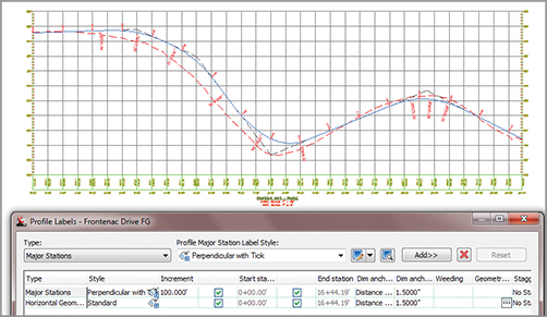
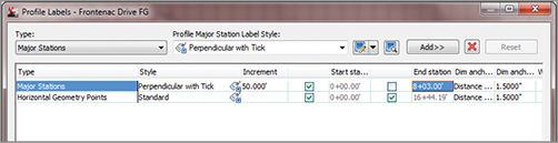
10. In the middle of the Profile Labels dialog, change the Increment value in the Major Stations row to 50, as shown in Figure 7-35. This modifies the labeling increment only, not the grid or other values.
Figure 7-35: Modifying the major station labeling increment

11. Click OK to close the Profile Labels dialog.
As you can see, applying labels one at a time could turn into a tedious task. After you learn about the types of labels available, you’ll revisit this dialog and look at the two buttons at the bottom for dealing with label sets.
Station Labels
Labeling along the profile at major, minor, and alignment geometry points lets you insert labels similar to a horizontal alignment. In this exercise, you’ll modify a style to reflect a plan-readable approach and remove the stationing from the first and last points along the profile:
1. Pick one of the station labels previously created and select Edit Label Group from the Modify panel to display the Profile Labels dialog.
2. Deselect the Start Station and End Station check boxes for the Major Stations label.
3. Change the value for the Start Station to 100 and the value of the End Station to 803, as shown in Figure 7-36.
Figure 7-36: Modifying the values of the starting and ending stations for the major labels
4. Click the icon next to Major Stations in the Style field to display the Pick Label Style dialog.
5. Select the Perpendicular With Tick Orientation.
6. Click OK to close the Profile Labels dialog. Instead of each station label being oriented so that it’s perpendicular to the profile at the station, all station labels are now oriented vertically along the top of the profile at the station.
By controlling the frequency, starting and ending station, and label style, you can create labels for stationing or for conveying profile information along a layout profile.
Line Labels
Line labels in profiles are typically used to convey the slope or length of a tangent segment. In this exercise, you’ll add a length and slope to the layout profile:
1. Pick the layout profile and select Edit Profile Labels from the Labels panel to display the Profile Labels dialog.
2. Change the Type field to the Lines option. The name of the Style drop-down menu changes to Profile Tangent Label Style. Select the Length and Percent Grade option.
3. Click the Add button, and then click OK to exit the dialog. The profile view should look like Figure 7-37.
Figure 7-37: A new line label applied to the layout profile
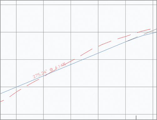
Where Is That Distance Being Measured?
The tangent slope length is the distance along the horizontal geometry between vertical curves. This value doesn’t include the tangent extensions. There are a number of ways to label this length; be sure to look in the Text Component Editor if you want a different measurement.
Curve Labels
Vertical curve labels are one of the most confusing aspects of profile labeling. Many people become overwhelmed rapidly because there’s so much that can be labeled and there are so many ways to get all the right information in the right place. In this quick exercise, you’ll look at some of the special label anchor points that are unique to curve labels and how they can be helpful:
1. Pick the layout profile and select Edit Profile Labels from the Labels panel to display the Profile Labels dialog.
2. Choose the Crest Curves option from the Type drop-down menu. The name of the Style drop-down menu changes. Select the Crest and Sag option.
3. Click the Add button to apply the label.
4. Choose the Sag Curves option from the Type drop-down menu. The name of the Style drop-down menu changes to Profile Sag Curve Label Style. Click Add to apply the same label style.
5. Click OK to close the dialog; your profile should look like Figure 7-38.
Figure 7-38: Curve labels applied with default values

Most labels are applied directly on top of the object being referenced. Because typical curve labels contain a large amount of information, putting the label right on the object can yield undesired results. In the following exercise, you’ll modify the label settings to review the options available for curve labels:
1. Pick the layout profile and select Edit Profile Labels from the Labels panel to display the Profile Labels dialog.
2. Scroll to the right in the middle of the dialog, and locate the Dim Anchor Opt column.
3. Change the Dim Anchor Opt value for the Sag Curves to Distance Below.
4. Change the Dim Anchor Val to 2′.
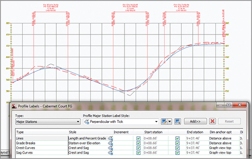
5. Change the Dim Anchor Val value for the Crest Curves to 2′ as well. Your dialog should look like the one shown in Figure 7-39.
Figure 7-39: Curve labels with distance values inserted
6. Click OK to close the dialog.
The labels can also be grip-modified to move higher or lower as needed, but you’ll try one more option in the following exercise:
1. Pick the layout profile and select Edit Profile Labels from the Labels panel to display the Profile Labels dialog.
2. Scroll to the right, and change both Dim Anchor Opt values for the Crest and Sag Curves to Graph View Top.
3. Change the Dim Anchor Val for both curves to –0.5′, and click OK to close the dialog. Your drawing should look like Figure 7-40.
Figure 7-40: Curve labels anchored to the top of the graph
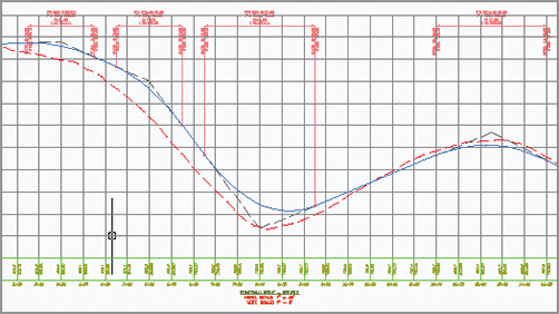
By using the top or bottom of the graph as the anchor point, you can apply consistent and easy labeling to the curve, regardless of the curve location or size.
Grade Breaks
The last label style typically involved in a profile is a grade-break label at PVI points that don’t fall inside a vertical curve, such as the beginning or end of the layout profile. Additional uses include things like water-level profiling, where vertical curves aren’t part of the profile information or existing surface labeling. In this exercise, you’ll add a grade-break label and look at another option for controlling how often labels are applied to profile data:
1. Open the Grade Break Profile Labels.dwg file.
2. Pick the red surface profile, and then select Edit Profile Labels from the Labels panel to display the Profile Labels dialog.
3. Choose Grade Breaks from the Type drop-down menu. The name of the Style drop-down menu changes. Select the Station Over Elevation style and click the Add button.
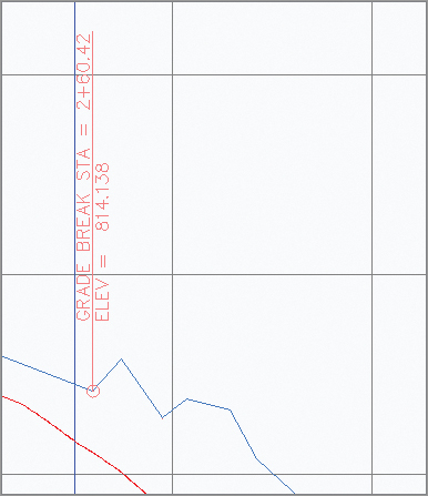
4. Click Apply, and drag the dialog out of the way to review the change. It should appear as in Figure 7-41.
Figure 7-41: Grade-break labels on a sampled surface
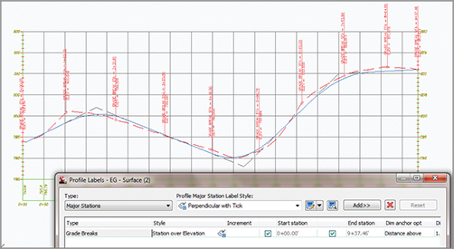
A sampled surface profile has grade breaks every time the alignment crosses a surface TIN line. Why wasn’t your view coated with labels?
5. Scroll to the right, and change the Weeding value to 50′.
6. Click OK to dismiss the dialog. Your profile should look like the one in Figure 7-42.
Figure 7-42: Grade-break labels with a 50′ Weeding value
Remember just as with almost every other label in Civil 3D, you can Ctrl+click a label to select a single one for deletion.
Weeding lets you control how frequently grade-break labels are applied. This makes it possible to label dense profiles, such as a surface sampling, without being overwhelmed or cluttering the view beyond usefulness.
As you’ve seen, there are many ways to apply labeling to profiles, and applying these labels to each profile individually could be tedious. In the next section, you’ll build a label set to make this process more efficient.
Staggering Profiles
When you are using Grade Breaks, there is an option in the Profile Labels dialog that will allow you to stagger the labels. The options as shown are Stagger Both Sides, No Staggering, Stagger To Right, and Stagger To Left.
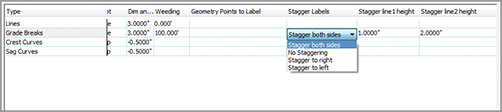
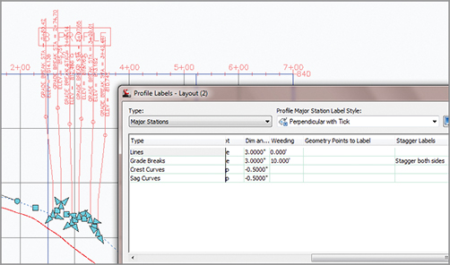
If you do not see all of the grade breaks, the Weeding value needs to be adjusted. In this example, the value is set to a default of 100′:
Setting a lower value, for example 10′, will show more grade breaks and you can see the staggered label effect.
In addition, you can set the stagger line lengths by entering values in the Stagger Line 1 Height and Stagger Line 2 Height text boxes.
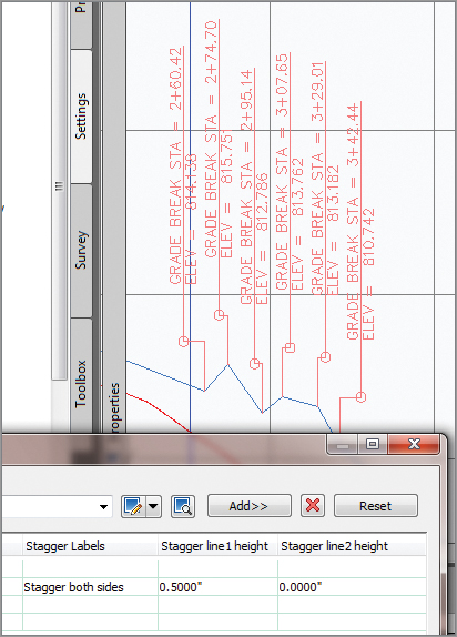
The Staggered labels can be gripped and dragged to new locations to suit your drawing.
Profile Label Sets
Applying labels to both crest and sag curves, tangents, grade breaks, and geometry with the label style selection and various options can be monotonous. Thankfully, Civil 3D gives you the ability to use label sets, as in alignments, to make the process quick and easy. In this exercise, you’ll apply a label set, make a few changes, and export a new label set that can be shared with team members or imported to the Civil 3D template. Follow these steps:
1. Delete the grade-break labels from the previous exercise.
2. Pick the layout profile, and then select Edit Profile Labels from the Labels panel to display the Profile Labels dialog.
3. Click the Import Label Set button near the bottom of the dialog to display the Select Style Set dialog.
4. Select the Standard option from the drop-down menu, and click OK.
5. Click OK again to close the Profile Labels dialog and see the profile view, as in Figure 7-43.
Figure 7-43: Profile with the Standard label set applied

6. Pick the layout profile and select Edit Profile Labels from the Labels panel to display the Profile Labels dialog.
7. Click Import Label Set to display the Select Style Set dialog.
8. Select the Complete Label Set option from the drop-down menu, and click OK.
9. Double-click the icon in the Style cell for the Lines label. The Pick Label Style dialog opens. Select the Length and Percent Grade option from the drop-down menu, and click OK.
10. Double-click the icon in the Style cell for the Crest label. The Pick Label Style dialog opens. Select the Crest and Sag option from the drop-down menu. Repeat this step for the Sag Curve label and click OK.
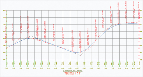
11. Click the Apply button, and drag the dialog out of the way, as shown in Figure 7-44, to see the changes reflected.
Figure 7-44: Establishing the Road Profile Labels set
12. Click the Save Label Set button to open the Profile Label Set dialog and create a new profile label set.
13. On the Information tab, change the name to Road Profile Labels. Click OK to close the Profile Label Set dialog.
14. Click OK to close the Profile Labels dialog.
15. On the Settings tab of Toolspace, select Profile Label Styles Label Sets. Note that the Road Profile Labels set is now available for sharing or importing to other profile label dialogs.
Sometimes You Don’t Want to Set Everything
Resist the urge to modify the beginning or ending station values in a label set. If you save a specific value, that value will be applied when the label set is imported. For example, if you set a station label to end at 15+00 because the alignment is 15+15 long, that label will stop at 15+00, even if the target profile is 5,000′ long!
Label sets are the best way to apply profile labeling uniformly. When you’re working with a well-developed set of styles and label sets, it’s quick and easy to go from sketched profile layout to plan-ready output.