Getting Started on the CAD Side

When you are getting ready to perform hydraulic or hydrologic computations using SSA, there are several steps that can be completed on the CAD side of Civil 3D.

You will use Civil 3D tools to find drainage points, catchment areas, and flow paths.

Water Drop

In any hydrologic system, it is important to know the direction water will flow on a surface. The Water Drop command is an excellent tool for determining where your outfall location should be. You will want to locate preliminary flow paths before defining the drainage basin.

To use the Water Drop command, select the surface you wish to analyze. Then select the Water Drop command from the Analyze panel of the Surface tab.

In the following exercise, you will use the Water Drop command on the existing site to determine the current flow pattern:

1. Open the WaterDrop.dwg file, which you can download from www.sybex.com/go/masteringcivil3d2012.

2. For this exercise, you will find it helpful to turn off object snaps and polar tracking.

3. Select the surface EG by clicking on any contour or portion of the boundary.

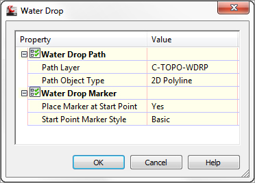
4. From the Analyze panel of the Surface tab, click Water Drop. The Water Drop settings will appear. Verify that the Place Marker At Start Point option is set to Yes, as shown in Figure 14-1. Click OK.

Figure 14-1: Water Drop command options

5. Get a feel for the site drainage by clicking on various areas throughout the site. There is no wrong place to click, as long as you are inside the surface boundary.

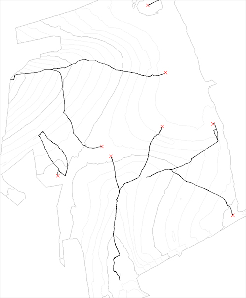
An X represents the place your cursor clicked. The place you click is a location on the surface where water hits the surface. You will see lines forming in the direction water flows from the area. If you see an X but no path, it could mean you are in a flat area or inside a small depression. After you click in several locations, your drawing will resemble Figure 14-2.

Figure 14-2: Surface with water drop paths

6. Click around as many places as you would like to examine. Press Esc when you finish.

The water drop paths that are created are polylines without any special intelligence. The next step demonstrates how to remove them if your surface model changes or you need to clear them from the screen.

7. (Optional) Select one of the X symbols and the water drop path. Be sure your surface is not selected. Right-click and choose Select Similar. All of the flow paths and corresponding Xs will be highlighted. Remove them by pressing Delete on your keyboard.

Catchments

The first step in any runoff computation is finding the area of the watersheds (also known as drainage basins or catchments) that contribute to the flow.

A new object type has been added to Civil 3D 2012: catchments. Catchments work with your surface models to determine the area draining to a point you specify. They are also used to find the drainage path within the catchment to compute time of concentration (Tc).

Catchment Groups

You must create a catchment group before creating catchments. Catchment groups are a way to separate predevelopment and postdevelopment watershed areas. Similar to sites, a catchment in one catchment group will not interfere with objects in another catchment group. Catchment groups do not interact with each other, allowing catchments from differing groups to overlay each other.

Catchment Creation

In Figure 14-3 you see a catchment with all its related features. You will need a grasp of the terminology used in the software before proceeding. It is useful to think about a hypothetical raindrop hitting the catchment to grasp what the various components represent.

Figure 14-3: A catchment with several flow path segments

Catchment Boundary The outline represents the catchment boundary, often called the basin divide or watershed boundary. This represents the outermost points of the catchment object. Any raindrops that hit inside this boundary will flow to the same point.

Discharge Point Toward the bottom of the boundary in Figure 14-3 is the discharge point. This is the main point of analysis used for the catchment. All raindrops that hit the basin ultimately end up at this location.

Hydraulically Most Distant Point Near the top of the catchment boundary in Figure 14-3 is a marker indicating the hydraulically most distant point. A raindrop that lands at this point will take the longest to arrive at the discharge point.

Catchment Flow Path In Figure 14-3, the catchment flow path is shown as a dashed line running through the catchment. This linear path represents the course the raindrop takes on its journey from the hydraulically most distant point to the discharge point. The catchment flow path is used to determine the slope and length for computing Tc for hydrology calculations.

Flow Path Segments By default, a flow path is created with an average slope through its overall length. Using flow path segments, you can break up the flow path into smaller pieces with the average slope computed per segment. Each segment can have different computation methods associated with them for Tc computations. The computation methods are as follows:

• SCS Shallow Concentrated Flow
• SCS Sheet Flow
• SCS Channel Flow

Time of Concentration Time of concentration is the time it takes for a drop of rain to travel from the hydraulically most distant point to the discharge point. The default method for determining this value is TR-55. Civil 3D uses the flow type, slope, and user-specified Manning’s roughness to determine the time. Alternately, you can input a user-defined time of concentration.

Catchment Options

You can choose to create a catchment from a surface model or by converting a closed polyline. You will get the best results when defining your catchment by converting a polyline to a catchment area. Manually delineate your watershed areas using the Water Drop command you used in the previous section as a guide.

Create Catchment From Object In most cases, this will be the method you should use for watershed creation. Use Create Catchment From Object if you have watershed data created ahead of time (i.e., from an imported GIS file or existing DWG). You will also need to use the Create Catchment From Object option for watersheds that are adjacent to your project’s limits of disturbance. Even if you choose to use an existing polyline as the catchment boundary, you can still use the surface model to determine the flow path location and slope.

Create Object From Surface Use the Create Catchment From Surface option if you have a well-formed surface model with adequate data for Civil 3D to compute the watershed area. Surface models with many flat areas, sparse data, or multiple hide boundaries will not work well for this tool. If you do not have good luck with this tool, don’t be surprised. Make sure the surface model used for catchment creation is complete before defining a catchment object. The catchment is not dynamically linked to the surface model; therefore, it will not update if changes are made to the surface model. If you are using the hydrology tool on an existing ground surface (predevelopment), make sure all surveyed shots and breaklines are added before proceeding. If you are using the tools on a proposed site (postdevelopment), make sure corridor surface models, grading surface models, and any proposed elevation data are pasted together in the surface model used for analysis.

In the following exercise, you will use multiple tools to delineate several watershed areas for a predeveloped site. You will also use the site characteristics to specify Manning’s roughness for SCS Sheet flow and SCS Channel flow. The site is covered in a dense grass.

1. Open the Catchment-1.dwg file, which you can download from this book’s web page.

2. For this exercise you will find it helpful to turn on the Insert object snap.

3. On the Analyze tab, locate the Ground Data panel. Choose Catchments ⇒ Create Catchment Group, as shown in Figure 14-4. Name the group Pre-developed. Click OK.

Figure 14-4: Accessing catchment tools from the Analyze tab

4. On the Analyze tab, locate the Ground Data panel. Choose Catchments ⇒ Create Catchment From Surface.

5. When you see the prompt Specify the Discharge Point:, select the insertion point of the storm structure labeled Existing Inlet (S).

6. When the Create Catchment From Surface dialog appears:

• Name the catchment South.
• Set the surface to Drainage GE-Survey.
• Click the select structure icon to set the Reference Pipe network structure to Existing Inlet (S).
• Alternately, you can right-click to pick structures from a list.
• Set Catchment Label Style to Name Area And Properties.
• Set Runoff Coefficient to 0.4. (This is the runoff coefficient used in the Rational method and will not affect our Tc value.)

If your dialog looks like Figure 14-5, click OK.

Figure 14-5: Create Catchment From Surface settings

7. After a moment, a red line representing the catchment boundary will form. Press Esc on your keyboard to dismiss the command.

8. On the Analyze tab, locate the Ground Data panel. Choose Catchments ⇒ Create Catchment From Object.

9. Select the closed polyline north of the first catchment. At the prompt Select a polyline on the uphill end to use as a flow path (or Press Esc to skip):, click the eastern end of the blue, dashed polyline that runs across the catchment.

10. In the Create Catchment From Object dialog that appears:

• Name the catchment North.
• Click the select structure icon to set the Reference Pipe network structure to Existing Inlet (N).
• Set Catchment Label Style to Name Area And Properties.
• Set Runoff Coefficient to 0.4.
• Uncheck Erase Existing Entities. Your dialog will now look like Figure 14-6a.
• Switch to the Flow Path tab.
• Set Flow Path Slopes to From Surface.
• Set Surface to Drainage GE-Survey.
• Your Flow Path tab will now look like Figure 14-6b. Click OK. Press Esc on your keyboard to exit the command.

Figure 14-6: Create Catchment From Object settings (a) and the Flow Path tab (b)

Your new catchment should resemble Figure 14-7.

Figure 14-7: The North catchment and flow path

11. Select the North catchment by clicking anywhere on the red boundary or on the dashed flow path line.

12. Right-click and select Edit Flow Segments, as shown in Figure 14-8.

Figure 14-8: Right-click to access Edit Flow Segments.

13. Panorama will appear showing the continuous path as SCS Shallow Concentrated Flow. Change Surface Type to Short Grass Pasture.

14. Click the plus sign in the upper-left corner to create a flow segment.

15. Create the new flow segment by clicking at the location on the flow line that crosses contour line 822′.

The new segment is placed in the Panorama listing from uphill to downhill. Segment 1 is the segment you just created and Segment 2 represents everything else downhill.

16. This new segment represents sheet flow. Change the flow type for Segment 1 to SCS Sheet Flow. Note the input fields change to accommodate this type of flow.

• Set the 2Yr-24Hr Rainfall value to 2.9″.
• Set the Manning’s Roughness value to 0.24.

The rainfall information used in this step was found in the PennDOT drainage design manual, which you can check for yourself at ftp://ftp.dot.state.pa.us/public/bureaus/design/PUB584/PDMChapter07A.pdf.

The Manning’s roughness for this area is based on coefficients for long grass found in the TR-55 document.

17. Click the plus sign and add the next segment at the abrupt bend in the flow path near the site boundary. This is where our flow enters a swale. For Segment 3, change Flow Type to SCS Channel Flow.

• Set the Manning’s Roughness value to 0.05.
• Set the Cross-Sectional Area value to 27 square feet.
• Set the Wetted Perimeter value to 28.2′.

Manning’s roughness was determined based on an earthen swale from TR-55. The cross-sectional area and wetted perimeter are site-specific measurements of the swale.

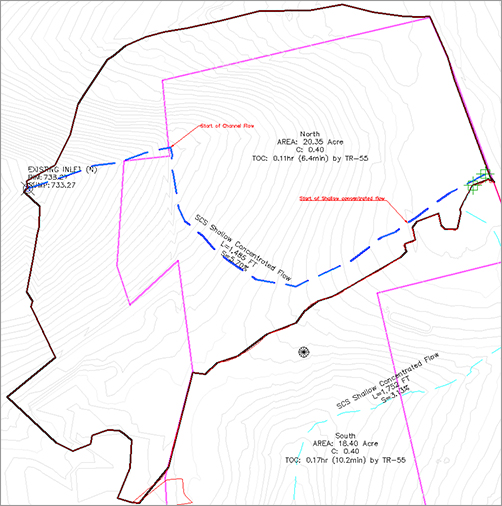
Your panorama should now look like Figure 14-9. You have used Civil 3D to compute the Tc for the north catchment.

Figure 14-9: Three flow segments with different characteristics

18. Save the drawing.

Catchment Areas to GIS

There are many situations where you will need to work with GIS data to send data to outside sources. You can use GIS data for anything from land uses to soil types. Luckily, Civil 3D contains all of Autodesk’s Map 3D program, allowing you to work with geographical data.

When catchments are exported to SSA from Civil 3D, the Tc, runoff coefficient, and area are exported as data only. However, you may be asked to provide ESRI Shape files (SHP) of your watershed areas.

To get physical geometry from Civil 3D, use parcels instead of catchments and then use GIS tools to move the data to SHP format:

1. Open the file Parcel Export.dwg, which you can download from this book’s web page.

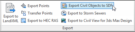
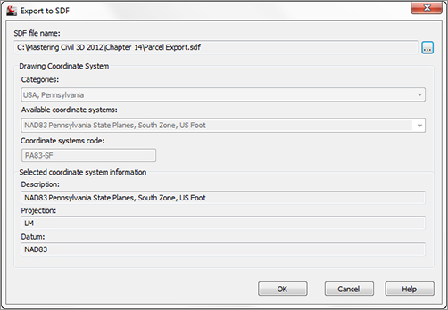
2. From the Export panel on the Output tab, click Export Civil Objects To SDF.

3. The SDF file will automatically be stored in the same folder as the DWG file you are working in. If you wish to change the location, click the ellipsis button. Click OK to confirm the coordinate system and create the SDF file.

The SDF file has been created, but to use it in SSA you must convert it to an SHP file. In the next steps you will be using the Map commands to perform the conversion. You will change to the Map part of the program by switching to the Planning And Analysis Workspace.

4. Change to the Planning And Analysis Workspace by clicking the gear icon in the lower-right corner of your Civil 3D screen. On the Data panel of the Home tab, click Connect.

5. On the left side of the Data Connect screen, click Add SDF Connection. On the right side of the dialog, click the browse icon beside the Source File field to browse to the file you created in step 3. Click Connect. No additional action is needed for the SDF data.

6. Next, highlight Add SHP Connection. Click the Folder icon and browse to the folder location where the project resides.

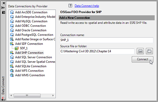
7. Click Connect. The folder you chose will be the destination for SHP files you will create in the steps that follow. No additional steps are needed in the Data Connect screen and you can click the X to close it.

8. Switch to the Create tab and locate the Feature Data Store panel. Click Bulk Copy.

9. In the From side of the screen on the left, set the Source to SDF_1. Scroll down the listing and put a check mark next to Parcels.

10. On the right side, set the To Target to SHP_1. Scroll down to where the command has automatically matched parcel information.

11. Double-click the field for Autogenerated_SDF_ID and rename it to ID. This step is necessary because the SHP file only supports property names containing fewer than 12 characters.

12. Click Copy Now. You will be prompted with a message warning you that the Bulk Copy operation cannot be undone. Click Continue Bulk Copy.

13. The Bulk Copy Results message should pop up, informing you that 13 objects were copied. Click OK.

14. Close the Bulk Copy dialog and close the drawing.

Exporting Pipes to SSA

When your catchments and your pipe networks are ready to analyze, switch to the Analyze tab and select Edit In Storm and Sanitary Analysis. You must have at least one pipe to export.

When you export, the pipe network information, inlets, pipes, and elevations convert over to SSA. Catchment data is shown with area, Tc, and runoff coefficient as data only. The graphic area that you define on the Civil 3D end is not needed.

When you first export a project over, SSA will ask if you would like to create a new project or open an existing project. If you are adding pipes to an existing network that has been analyzed in SSA, click the Open Existing Project radio button and browse to the location of your stored SPF file.

When you create a new project, SSA does a few grunt-work things for you. First, it converts all your junctions and pipes to the SSA format (via Hydraflow’s STM file, oddly enough) and asks if you would like to save the log file. Generally, saving the log file is not necessary unless you are having difficulty importing certain objects. In most cases, you can click No to continue.

Once you are in the SSA interface, you can access your active project by clicking the Plan View tab at the top of the window. You will see your DWG file as an underlay to the project you are working on.

How Does SSA Decide What’s an Inlet and What’s a Manhole?

Buried deep in the bowels of your command settings are the Part Matchup Settings. On the Settings tab, choose Pipe Networks ⇒ Commands and double-click the EditInSSA option. Once you are there, expand the Storm Sewers Migration Defaults area.

Click the Part Matching Defaults field. Click the ellipsis to enter the Part Matchup Settings dialog.

The Import tab handles how parts from SSA or Hydraflow behave on the way into Civil 3D. The Export tab handles how SSA or Hydraflow handles parts from Civil 3D. As you can tell from poking around here, there isn’t always a perfect match for every part you use.

There are a few quirks and limitations with the intended SSA workflow:

• Pipe networks that contain parts from multiple-part families (for example, a pipe network may contain a part from the HDPE family and another part from the Concrete family) will reimport back into Civil 3D with only one part family.
• To prevent SSA and Civil 3D from changing your pipe sizes, make a single part family for all circular pipes. Be sure that the “master” part family contains all possible sizes. Once it is reimported back to Civil 3D, use Swap Part to change back to the original part family type.
• For advanced users, there is a super-secret XML file located in C:Program Files(x86)AutodeskSSA 2012SamplesPart Matching. For more information about using and editing this file, see the Part Matching help file.
• Culverts are treated the same as a single pipe in SSA. Once you export a culvert into SSA, you’ll need to set entrance and exit conditions.

A little part tune-up will be needed after the round-trip; however, the time savings in using the export commands are still very much worth it.