
Once a surface is created, you can display information in a number of ways. The most common so far has been contours and triangles, but those are the basics. By using varying styles, you can show a large amount of data with one single surface. Not only can you do simple tasks such as adjust the contour interval, but Civil 3D can apply a number of analysis tools to any surface:
Contours Allows the user to specify a more specific color scheme or linetype as opposed to the typical minor-major scheme. Commonly used in cut-fill maps to color negative colors one way, positive contours another, and the balance or zero contours yet another color.
Elevations Creates bands of color to differentiate various elevations. You can use this tool to create a simple weighted distribution to help in development of marketing materials, hard-coded elevations to differentiate floodplain and other elevation-driven site concerns, or ranges to help a designer understand the earthwork involved in creating a finished surface.
Direction Analysis Draws arrows showing the normal direction of the surface face. This tool is typically used for aspect analysis, helping site planners review the way a site slopes with regard to cardinal directions and the sun.
Slopes Analysis Colors the face of each triangle on the basis of the assigned slope values. Although a distributed method is the normal setup, a common use is to check site slopes for compliance with Americans with Disabilities Act (ADA) requirements or other site slope limitations, including vertical faces (where slopes are abnormally high).
Slope Arrows Displays the same information as a slope analysis, but instead of coloring the entire face of the TIN, this option places an arrow pointing in the downhill direction and colors that arrow on the basis of the specified slope ranges.
User-Defined Contours Refers to contours that typically fall outside the normal intervals. These user-defined contours are useful to draw lines on a surface that are especially relevant but don’t fall on one of the standard levels. A typical use is to show the normal pool elevation on a site containing a pond or lake.
Contouring Basics
Contouring is the standard surface representation on which land development plans are built. But in earlier programs such as Autodesk’s Land Development, changing the contouring interval was akin to pulling teeth. With the use of styles in Civil 3D, you can have any number of styles prebuilt to allow you to quickly and painlessly change how contours are displayed. In this example, you’ll copy an existing surface contouring style and modify the interval to a setting more suitable for commercial site design review:
1. Open the SurfaceContours.dwg file. This surface is currently displayed with a 5″ minor contour and 25″ major contour.
2. Select the surface by picking any contour or the boundary, and then click the Surface Properties button on the Modify panel. The Surface Properties dialog appears.
3. On the Information tab, click the down arrow next to the Style Editor button. Select the Copy Current Selection option to display the Surface Style dialog.
4. On the Information tab, change the Name field to Contours 0.25″ and 1″ and remove the description in place.
5. Switch to the Contours tab and expand the Contour Intervals property, as shown in Figure 4-36.
Figure 4-36: The expanded Contour Intervals setting
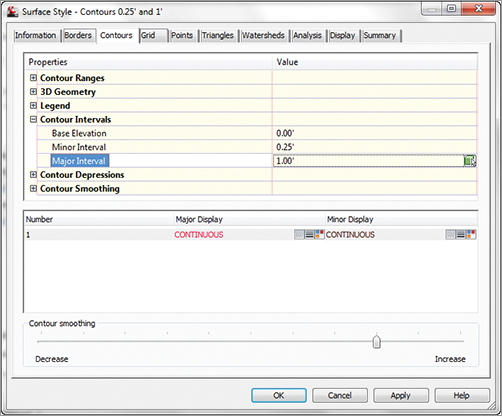
6. Change the Minor Interval value to 0.25″ and press ↵. The Major Interval value will jump to 1.25″, maintaining the ratio that was previously in place.
7. Change the Major Interval value to 1.0″ and press ↵.
8. Expand the Contour Smoothing property (you may have to scroll down). Select a Smooth Contours value of True, which activates the Contour Smoothing slider bar near the bottom. Don’t change this Smoothing value, but keep in mind that this gives you a level of control over how much Civil 3D modifies the contours it draws.
9. Click OK to close this dialog and then click OK again to close the Surface Properties dialog.
Surface vs. Contour Smoothing
Remember, contour smoothing is not surface smoothing. Contour smoothing applies smoothing at the individual contour level but not at the surface level. If you want to make your surface contouring look fluid, you should be smoothing the surface.
The surface should be rendered faster than you can read this sentence even with the incredibly tight contour interval you’ve selected. This style doesn’t make much sense on a site like this one, but it can be used effectively on something like a commercial site or highway entrance ramp where the low surface slope values make 1″ contours close to meaningless in terms of seeing what is going on with the surface.
You skipped over one portion of the surface contours that many people consider a great benefit of using Civil 3D: depression contours. If this option is turned on via the Contours tab, ticks will be added to the downhill side of any closed contours leading to a low point. This is a stylistic option, and usage varies widely.
Now let’s look at a few of the other options and areas you ignored in creating this style. There are some interesting changes from many other Civil 3D objects, as you can see in the component listing in Figure 4-37.
Figure 4-37: Listing of surface style components in the Plan direction

Under the Component Type column, Points, Triangles, Border, Major Contour, Minor Contour, User Contours, and Gridded are standard components and are controlled like any other object component. The plan (aka 2D), model (aka 3D), and section views are independent, and surfaces are one of the objects where different plan and model views are common. The Directions, Elevations, Slopes, and Slope Arrows components are unique to surface styles. Note that the Layer, Color, and Linetype fields are grayed out for these components. Each of these components has its own special coloring schemes, which we’ll look at in the next section.
Elevation Banding
Displaying surface information as bands of color is one of the most common display methods for engineers looking to make a high-impact view of the site. Elevations are a critical part of the site design process, and understanding how a site flows in terms of elevation is an important part of making the best design. Elevation analysis typically falls into two categories: showing bands of information on the basis of pure distribution of linear scales or showing a lesser number of bands to show some critical information about the site. In this first exercise, you’ll use a pretty standard style to illustrate elevation distribution along with a prebuilt color scheme that works well for presentations:
1. Open the SurfaceAnalysis.dwg file.
2. Pick the surface on your screen.
3. Select Surface Properties from the Surface tab on the Modify panel. The Surface Properties dialog appears.
4. On the Information tab, change the Surface Style field to Elevation Banding (3D).
5. Switch to the Analysis tab.
6. Click the Run Analysis arrow in the middle of the dialog to populate the Range Details area.
7. Click OK to close the Surface Properties dialog.
8. From the View control, select SW Isometric.
9. Zoom in if necessary to get a better view.
10. From the Visual Style control, select the Conceptual option to see a semi-rendered view that should look something like Figure 4-38.
Figure 4-38: Conceptual view of the site with the Elevation Banding style

AutoCAD Visual Styles
The triangles seen are part of the view style and can be modified via the Visual Styles Manager. Turning the Edge mode off will leave you with a nicely gradated view of your site. You can edit the visual style by clicking the View control at the upper left of your drawing screen. You can also select View Visual Styles Visual Style Manager on the main menu.

You’ll use a 2D elevation to clearly illustrate portions of the site that cannot be developed. In this exercise, you’ll manually tweak the colors and elevation ranges on the basis of design constraints from outside the program:
1. Click the View control and select Top.
2. Click the Visual Style control and select 2D Wireframe.
This site has a limitation placed in that no development can go below the elevation of 790. Your analysis will show you the areas that are below 790, a buffer zone to 791, and then everything above that.
3. Select the surface, right-click, and choose the Surface Properties option. The Surface Properties dialog appears.
4. On the Information tab, change the Surface Style field to Zoning.
5. Double-clicking in the Minimum and Maximum Elevations fields allows for direct editing. Double-clicking the Color Swatch field allows for manual picking. Modify your surface properties to match Figure 4-39. (The colors are red, yellow, and green from top to bottom, respectively.)
Figure 4-39: The Surface Properties dialog after manual editing

6. Click OK to exit the dialog.
Understanding surfaces from a vertical direction is helpful, but many times, the slopes are just as important. In the next section, you’ll take a look at using the slope analysis tools in Civil 3D.
Slopes and Slope Arrows
Beyond the bands of color that show elevation differences in your models, you also have tools that display slope information about your surfaces. This analysis can be useful in checking for drainage concerns, meeting accessibility requirements, or adhering to zoning constraints. Slope is typically shown as areas of color as the elevations were or as colored arrows that indicate the downhill direction and slope. In this exercise, you’ll look at a proposed site grading surface and run the two slope analysis tools:
1. Open the SurfaceSlopes.dwg file.
2. Select the surface in the drawing and click the Surface Properties button on the Modify panel. The Surface Properties dialog appears.
3. On the Information tab, change the Surface Style field to Slope Banding (2D).
4. Change to the Analysis tab.
5. Change the Analysis Type drop-down list to Slopes.
6. Change the Number field in the Ranges area to 5 and click the Run Analysis button. The Range Details area will populate.
7. Click OK to close the dialog. Your screen should look like Figure 4-40.
Figure 4-40: Slope color banding analysis

The colors are nice to look at, but they don’t mean much, and slopes don’t have any inherent information that can be portrayed by color association. To make more sense of this analysis, add a table:
1. Select the surface again and select the Add Legend button on the Labels & Tables panel.
2. Type S at the command line to select Slopes, and press ↵.
3. Press ↵ again to accept the default value of a Dynamic legend.
4. Pick a point on screen to draw the legend, as shown in Figure 4-41.
Figure 4-41: The Slopes legend table
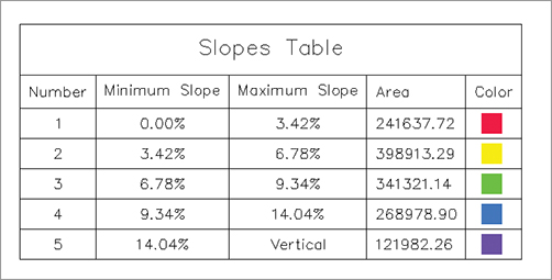
By including a legend, you can make sense of the information presented in this view. Because you know what the slopes are, you can also see which way they go.
1. Select the surface and click the Surface Properties button on the Modify panel. The Surface Properties dialog appears.
2. On the Information tab, choose Slope Arrows from the Surface Style drop-down list.
3. Change to the Analysis tab.
4. Choose Slope Arrows from the Analysis Type drop-down list.
5. Change the Number field in the Ranges area to 5 and click the Run Analysis button.
6. Click OK to close the dialog.
The benefit of arrows is in looking for “birdbath” areas that will collect water. These arrows can also verify that inlets are in the right location, as shown in Figure 4-42. Look for arrows pointing to the proposed drainage locations and you’ll have a simple design-verification tool.
Figure 4-42: Slope arrows pointing to a proposed inlet location

With these simple analysis tools, you can show a client the areas of their site that meet their constraints. Visually strong and simple to produce, this is the kind of information that a 3D model makes available. Beyond the basic information that can be represented in a single surface, Civil 3D also contains a number of tools for comparing surfaces. You’ll compare this existing ground surface to a proposed grading plan in the Comparing Surfaces section.
Visibility Checker
New to Civil 3D 2012 are some tools that allow you to see issues that might occur even before dirt is moved. The Zone of Visual Influence tool allows you to explore what-if scenarios. In this example, a 40′ tower has been proposed for the site. A concerned neighbor wants to make sure that it won’t obstruct their scenic view. We want to check it from the proposed surface:
1. Open VisibilityCheck.dwg.
2. Click on the proposed surface. This is the one with the blue solid contours.
3. In the Tin Surface tab and Analyze panel, select Visibility CheckZone of Visual Influence.
4. Using the Intersection osnap, select the center of the proposed tower located on the lower portion of the site.
5. Type 40↵ to set the tower height to 40′.
6. Select an intersection of the cyan color house located at the upper right of the site.
The drawing now has bands of color. The green color indicates that the object is completely visible, the yellow color indicates that the object is partially visible, and the red color indicates that the object is not visible.
So in our example, the homeowner on the upper right will be happy to know that the proposed 40′ tower will not appear in their view.
The next example will use the Point to Point tool.
1. Using the same drawing as before, zoom to the intersection of Syrah Way and Cabernet Court where you will see a car. We want to check the sight distance.
2. If it is not already selected, click on the Composite surface.
3. From the Tin Surface tab and Analyze panel, select Visibility CheckPoint to Point.
4. At the Specify height of eye: prompt, type 3.5↵. This sets the height of a driver’s eye while sitting in a typical car.
5. At the Specify location of eye: prompt, click where the driver would normally be seated in the vehicle.
6. The next prompt (Specify height of target:), is asking what the view height is that a driver can see while seated in the vehicle. Type 6↵.
7. Click along the path where oncoming cars would be seen. An arrow is drawn on the screen. If the arrow is green, it means that the view is unobstructed. If the arrow is red, it indicates that the view is obstructed and the command prompt will tell you where the obstruction occurs.
Unfortunately, these Visual tools are not dynamic; if you change the profile, you will need to re-run the visual tools. Perhaps next release.