Before any project-specific data is imported, there is a bit of onetime setup that will improve the translation between the field and the office.
Your survey database defaults, equipment database, linework code set, and the figure prefix database should be in place before you import your first survey. You can find the location of these files by going to the Survey tab in Toolspace and clicking the Survey User Settings button in the upper-left corner. The dialog shown in Figure 2-1 opens.
Figure 2-1: Survey User Settings dialog

It is common practice to place these files on a network server so your organization can share them. Change the paths in this dialog and they will “stick” regardless of which drawing you have open.
Survey Database Defaults
When you first set up your survey settings, it is a good idea to create a test database for setting the survey database defaults. To create the test database, right-click Survey Databases on the Survey tab and select New Local Survey Database. Name the new database Test, and click OK to continue. Right-click the new Test database and select Edit Survey Database Settings.
Once you set your desired defaults for units, precision, and other options, click the Export Settings To A File button. Then save the settings to the folder specified in the Survey User Settings dialog (see Figure 2-2).
Figure 2-2: Survey Database settings

The Survey User Settings dialog contains these settings:
Units This section is where you set your master coordinate zone for the database. If you insert any information in the database into a drawing with a different coordinate zone set, the program will automatically translate that data to the drawing coordinate zone. Your coordinate zone units will lock the distance units in the Units section. You can also set the angle, direction, temperature, and pressure here.
Precision This section is where you define and store the precision information of angles, distance, elevation, coordinates, and latitude and longitude.
Measurement Type Defaults This section lets you define the defaults for measurement types, such as angle type, distance type, vertical type, and target type.
Measurement Corrections This section is used to define the methods (if any) for correcting measurements. Some data collectors allow you to make measurement corrections as you collect the data, so that needs to be verified, because double correction applications could lead to incorrect data.
Traverse Analysis Defaults This section is where you choose how you perform traverse analyses and define the required precision and tolerances for each. There are four types of 2D traverse analyses: Compass Rule, Transit Rule, Crandall Rule, and Least Squares Analysis.
There are also two types of 3D traverse analyses: Length Weighted Distribution and Equal Distribution.
Least Squares Analysis Defaults This section is where you set the defaults for a least squares analysis. You only need to change settings here if least squares analysis is the method you will use for your horizontal and/or vertical adjustments.
Survey Command Window The Survey Command window is the interface for manual survey tasks and for running survey batch files. This section lets you define the default settings for this window.
Error Tolerance Set tolerances for the survey database in this section. If you perform an observation more than one time and the tolerances set within are not met, an error will appear in the Survey Command window and ask you what action you want to take.
Extended Properties This section defines settings for adding extended properties to a survey LandXML file. Extended properties are useful for certain types of surveys, including Federal Aviation Administration (FAA)–certified surveys.
To delete your test database, you will need to close the database from the Survey tab. To do so, locate the database in the Survey tab. Right-click on it and select Close Survey Database. Using Windows Explorer, you can then browse to the working folder containing the database and delete it. There is no way to delete a survey database from within the software.
The Equipment Database
The equipment database is where you set up the various types of survey equipment that you are using in the field. Doing so allows you to apply the proper correction factors to your traverse analyses when it is time to balance your traverse. Civil 3D comes with a sample piece of equipment for you to inspect to see what information you will need when it comes time to create your equipment. The Equipment Properties dialog provides all the default settings for the sample equipment in the equipment database. Expand the Equipment Databases Sample branches, right-click Sample, and select Manage Equipment Database to access this dialog in Toolspace, as shown in Figure 2-3.
Figure 2-3: Equipment Database Manager

You will want to create your own equipment entries and enter the specifications for your particular total station. Add a new piece of equipment to the database by clicking the plus sign at the top of the Equipment Database Manager window. If you are unsure of the settings to enter, refer to the user documentation that you received when you purchased your total station.
The Figure Prefix Database
The figure prefix database is used to translate descriptions in the field to lines in CAD. These survey-generated lines are called figures. If a description matches a listing in the figure prefix database, the figure is assigned the properties and style dictated therein (see Figure 2-4).
Figure 2-4: Figure Prefix Database Manager

The Figure Prefix Database Manager contains these columns:
Breakline This column specifies whether the figure should be used as a breakline during surface creation. To dispel common misconceptions about this option, you should know that a figure flagged as a breakline still needs to be added to the surface definition by the user (i.e., no automatic breaklines appear in a surface), and a figure not flagged as a breakline can still be added to the surface. This option sets the Breakline Option to Yes automatically when you right-click the Figures listing and select Create Breaklines.
Lot Line This column specifies whether the figure should behave as a parcel segment. If a closed area is formed with figures of this kind, a parcel is also formed.
Layer This column specifies the layer that the figure will reside on when inserted into the drawing. If the layer already exists in the drawing, the figure will be placed on that layer. If the layer does not exist in the drawing, the layer will be created and the figure placed on the newly created layer.
Style This column specifies the style to be used for each figure. The style contains the linetype and color of the figure. If the style exists in the current drawing, the figure will be inserted using that style. If the style does not exist in the drawing, the style will be created with the standard settings and the figure will be placed in the drawing according to the settings specified with the newly created style.
Site This column specifies which site the figures should reside on when inserted into the drawing. As with previous settings, if the site exists in the drawing, the figure will be inserted into that site. If the site does not exist in the drawing, a site will be created with that name and the figure will be inserted into the newly created site.
Next you’ll explore these settings in a practical exercise. You’ll use the styles created in the previous exercise:
1. Open the drawing figure prefix library.dwg, which you can download from this book’s webpage, www.sybex.com/go/masteringcivil3d2012.
2. In the Survey tab of Toolspace, right-click Figure Prefix Databases and select New. The New Figure Prefix Database dialog opens.
3. Enter Mastering Civil 3D in the Name text box, and click OK to dismiss the dialog. Mastering Civil 3D will now be listed under the Figure Prefix Databases section in the Survey tab on Toolspace.
4. Right-click the newly created Mastering Civil 3D figure prefix database and select Manage Figure Prefix Database. The Figure Prefix Database Manager will appear.
5. Select the white + symbol in the upper-left corner of the Figure Prefix Database Manager to create a new figure prefix.
6. Click the SAMPLE name and rename the figure prefix to EP (for Edge of Pavement).
7. Check the No box in the Breakline column to change it to Yes so the figure will be treated as a breakline. Leave the box in the Lot Line column unchecked, so the figure will not be treated as a parcel segment.
8. Under the Layer column, select V-SURV-FIGR.
9. Under the Style column, select EP.
10. Under the Site column, leave the name of the site set to Survey Site.
11. Complete the Figure Prefixes table with the values shown in Table 2-1.
12. Click OK to dismiss the Figure Prefix Database Manager.
Table 2-1: Figure settings

The Linework Code Set Database
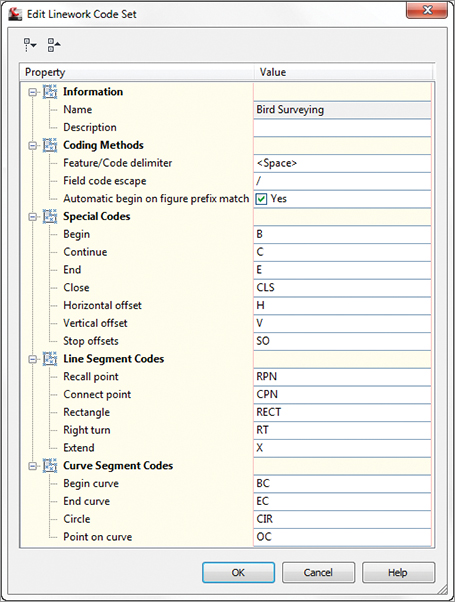
The linework code set (Figure 2-5) lists what designators are used to start, stop, continue, or add additional geometry to lines. For example, the B code that is typically used to begin a line can be replaced by a code of your choosing, a decimal (.) can be used for a right-turn value, and a minus sign (–) can be used for a left-turn value. Linework code sets allow a survey crew to customize their data collection techniques based on methods used by various types of software not related to Civil 3D.
Figure 2-5: The Edit Linework Code Set dialog
You Do Not Need Linework Codes in Your Survey to Generate Lines!
There is a setting in the linework code set called Automatic Begin On Figure Prefix Match (as you can see in Figure 2-5). If you select this option, lines will start when a shot description matches one of your figure prefixes (such as EP or CL in Figure 2-4), with no additional coding needed.
Depending on your survey department’s method for picking up linework, Automatic Begin On Figure Prefix Match can be a good thing or a bad thing. If the survey crew has fastidiously collected each line with its own name, such as CL1, CL2, EP1, EP2, and so on with no repeats, it can work well. If they use start and stop codes but reuse line names throughout the survey, it can produce figures that connect unintentionally.
The Main Event: Your Project’s Survey Database
Now that you know how to get everything set up, you are probably eager to get some real, live data into your drawing.
First, set your survey working folder to your desired survey storage location. The Civil 3D survey database is a set of external Microsoft SQL Server Compact database files that reside in your survey working folder. By default, this folder is located in C:Civil 3d Projects.
To set the survey working folder, right-click on Survey Databases and select Set Working Folder, as shown in Figure 2-6.
Figure 2-6: Set the survey working folder.
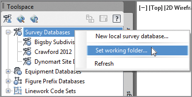
In the current version of Civil 3D, this is a different, independent setting from the working folder for data shortcuts. Most folks want this on a network location, tucked neatly into the survey folder for the project.
Keep in mind that the survey database is version specific. You can open a 2011 database in 2012, but once it has been converted, there is no going back.
To create a survey database, you can either right-click and select New Local Survey Database as mentioned earlier, or you can select Import Survey Data from the Home tab’s Create Ground Data panel.
The contents of a survey database are organized into the following categories:
Import Events Import events provide a framework for viewing and editing specific survey data, and they are created each time you import data into a survey database. The default name for the import event is the same as the imported filename. The Import Event collection contains the networks, figures, and survey points that are referenced from a specific import command, and provides an easy way to remove, re-import, and reprocess survey data in the current drawing.
Networks A survey network is a collection of related data that is collected in the field. The network consists of setups, control points, noncontrol points, known directions, observations, setups, and traverses. A network must be created in a survey database before any data can be imported. A survey database can have multiple networks. For example, you can use different networks for different phases of a project. If working within the same coordinate zone, some users have used one survey database with many networks for every survey that they perform. This is possible because individual networks can be inserted into the drawing simply by dragging and dropping the network from the Survey tab in Toolspace into the drawing. You can hover your cursor over any Survey Network component in the drawing to see information about that component and the survey network. You can also right-click any component of the network and browse to the observation entry for that component.
Network Groups Network groups are collections of various survey networks within a survey database. These groups can be created to facilitate inserting multiple networks into a drawing at once simply by dragging and dropping.
Figures Figures are the linework created by codes and commands entered into the raw data file during data collection. The figure names typically come from the descriptor or description of a point.
Figure Groups Similar to network groups, figure groups are collections of individual figures. These groups can be created to facilitate quick insertion of multiple figures into a drawing.
Survey Points One of the most basic components of a survey database, points form the basis for each and every survey. Survey points look just like regular Civil 3D point objects, and their visibility can be controlled just as easily. However, one major difference is that a survey point cannot be edited within a drawing. Survey points are locked by the survey database, and the only way of editing is to edit the observation that collected the data for the point. This provides the surveyor with the confidence that points will not be accidentally erased or edited. Like figures, survey points can be inserted into a drawing by either dragging and dropping from the Survey tab of Toolspace or by right-clicking Surveying Points and selecting the Points Insert Into Drawing option.
Survey Point Groups Just like network groups and figure groups, survey point groups are collections of points that can be easily inserted into a drawing. When these survey point groups are inserted into the drawing, a Civil 3D point group is created with the same name as the survey point group. This point group can be used to control the visibility or display properties of each point in the group.
In the following exercise, you’ll create an import event and import an ASCII file with survey data. The survey data includes linework.
1. Create a new drawing from the _AutoCAD Civil 3D (Imperial) NCS.dwt template file.
2. From the Home tab, in the Create Ground Data panel of the Ribbon, click Import Survey Data to open the Import Survey Data wizard.
3. Click Create New Survey Database.
4. Enter Roadway as the name of the folder in which your new database will be stored. Click OK. Roadway is now added to the list of survey databases.
5. Click Edit Survey Database Settings and verify the units are set to US Foot. Click OK to dismiss the dialog.
6. Click Next.
7. Set the Data Source Type drop-down to Point File.
8. Click the Add Files button on the right side of the Selected File text box, and browse to the import points.txt file, which you can download from this book’s webpage, www.sybex.com/go/masteringcivil3d2012.
9. Click Open and the name will be listed in the dialog as shown in Figure 2-7.
Figure 2-7: Select the correct file type, file, and format in the Import Survey Data wizard.

10. Under Specify Point File Format, scroll through the list until you find PNEZD (Comma Delimited). Highlight the format. The preview will show that the correct data type is selected. Click Next to continue.
11. Click Create New Network. Enter the name Roadway as the name of the network. Click OK. Click Next to continue.
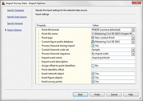
12. Verify that your import options match what is shown in Figure 2-8. Click Finish.
Figure 2-8: The Import Options page in the Import Survey Data wizard
The data is imported and the linework is drawn; however, the building is missing the left side. The following steps will resolve this issue:
1. Continue working in the drawing from the previous exercise. In the Survey tab, select Survey Databases, and then select Roadway, Networks, Roadway, and Non-Control Points.
2. Right-click and select Edit to bring up the Non-Control Points Editor palette in Panorama.
3. Scroll to the bottom of the point list and notice the last line in the file describing point number 34.
4. Move your cursor to the right of the description and type CLS, as shown in Figure 2-9. This is the default Close Figure command.
Figure 2-9: Editing the import event to add the CLS command and close the building geometry

5. Click the check box in the upper right of the palette to apply changes and save your edits. A warning dialog will appear. Click Yes to apply your changes.
6. Select Survey Databases, choose Roadway, click Import Events, and select import points.txt. Right-click import points.txt, and select Process Linework to bring up the Process Linework dialog.
7. Click OK to reprocess the linework with your updated point description. The building figure line and your drawing should look something like Figure 2-10.
Figure 2-10: After editing and reprocessing the linework

Editing the Surveyed Point?
Many surveyors will cringe at this new ability to easily modify the drawing data without updating the source files from the field survey. We think this is an improvement in that you can create drawings that accurately reflect personal field observations without modifying the legal record that is the original survey data.
“Mommy, Where Does Survey Data Come From?”
The type of file you will end up bringing into Civil 3D largely depends on your data collector. Civil 3D can import a number of different file formats, but file types vary in what information they can place in the survey database:
ASCII Text File Most commonly, this is a PNEZD file format (Point Number, Northing, Easting, Elevation, Description). This type of file can produce linework, but every shot is listed as a noncontrol point. The file extension on this type of file may be shown as .txt, .csv, or something else.
LandXML Contains raw data, points, linework, and even point groups and figure groups. LandXML is the most efficient method for transferring the entirety of a survey database if needed by an outside organization.
FBK (Field Book Format) Can contain raw data, linework, and setup information. FBK is a specially formatted text-based file that was the only format option for creating linework in legacy Autodesk products. In the current release, FBK is no longer king, but it is still a widely used format in many data collectors.
Let’s look at some of the manufacturers in the data collector market:
Trimble Trimble has two major offerings: the Trimble TCS Survey Controller and the Trimble SCS900 Site Controller. Both of these data collectors interact directly with Civil 3D via a freely available download called Trimble Link from the Trimble website. This download will add a Trimble Ribbon tab to Civil 3D and allow uploading and downloading of data directly using both data collectors as well as Trimble Site Vision software. Trimble Link will take a JOB file (the default file format for Trimble), convert it to an FBK transparently, create a new survey network in a new or existing database, and import the FBK into that newly created network, all in one step. You can download the software from www.trimble.com/link_ts.asp?Nav=Collection-63438.
TDS Now a division of Trimble, Survey Pro is one of the most popular data collection software packages on the market today. The TDS RAW or RW5 file format is the format on which other data collector manufacturers base their RAW data files. To convert from a TDS RAW data file to an FBK, users must either purchase TDS ForeSight DXM or use TDS Survey Link, which is included in your Civil 3D install. You can initiate Survey Link by typing STARTSURVEYLINK on the command line, or by selecting Survey Data Collection Data Link from the Create Ground Data panel on the Home tab.
Leica The Leica System 1200 data collectors can be integrated with Civil 3D via the use of Leica X-Change. Leica X-Change allows for the import of Leica data and conversion to the FBK format, as well as export options for Leica System 1200 collectors. You can download the software from www.leica-geosystems.com/corporate/en/downloads/lgs_page_catalog.htm?cid=239.
MicroSurvey MicroSurvey has an advantage not shared by any other data collector in this list: It has the ability to directly export an FBK from the data collector. However, if users demand a conversion process, the MicroSurvey RAW data file is based on TDS RAW data, and it can be converted using the included TDS Survey Link.
Carlson Like Trimble, Carlson offers a freely downloadable plug-in for Civil 3D. Carlson Connect allows for direct import and export to Carlson SurvCE data collectors as well as a conversion option for drawings containing Carlson point blocks. You can download the software by going to http://update.carlsonsw.com/updates.php and selecting Carlson Connect as the product you are seeking.
Under the Hood in Your Survey Database
Once you import survey data, Civil 3D will help you make sense of it by organizing the data into groups, as shown in Figure 2-11:
Figure 2-11: A typical survey database network with data
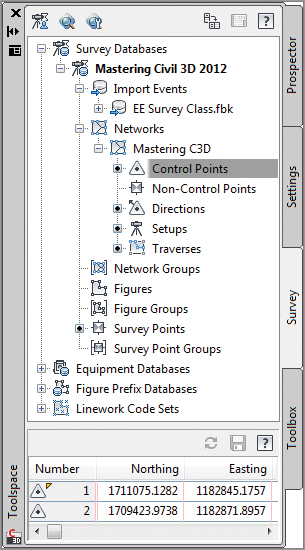
Control Points Control points are typically points in your data that have a high confidence factor. These are usually benchmarks or other known points used to lock the survey into its geographical location.
Non-Control Points Noncontrol points are also stored in the survey database. Keyed-in points; GPS-collected points, such as those located by real-time kinematic (RTK) GPS; and any point brought in through an ASCII file will appear as noncontrol points.
Directions The direction from one point to another must be manually entered into the data collector for the direction to show up later in the survey network for editing. The direction can be as simple as a compass shot between two initial traverse points that serves as a rough basis of bearings for a survey job.
Setups The setup is typically where the meat of the data is found, especially when working with conventional survey equipment. Every setup, as well as the points (side shots) located from that setup, can be found. Setups will contain two components: the station (or occupied point) and the backsight. Setups, as well as the observations located from the setup, can be edited. The interface for editing setups is shown in Figure 2-12. Angles and instrument heights can also be changed in this dialog.
Figure 2-12: Setups and observations can be changed in the Setups Editor.

Traverses
The Traverses section is where new traverses are created or existing ones are edited. These traverses can come from your data collector, or they can be manually entered from field notes via the Traverse Editor, as shown in Figure 2-13. You can view or edit each setup in the Traverse Editor, as well as the traverse stations located from that setup.
Figure 2-13: The Traverse Editor

Once you have defined a traverse, you can adjust it by right-clicking its name and selecting Traverse Analysis. You can adjust the traverse either horizontally or vertically, using a variety of methods. The traverse analysis can be written to text files to be stored, and the entire network can be adjusted on the basis of the new values of the traverse, as you’ll do in the following exercise:
1. Create a new drawing from the _AutoCAD Civil 3D (Imperial) NCS.dwt template file.
2. Navigate to the Survey tab of Toolspace.
3. Right-click Survey Databases and select New Local Survey Database. The New Local Survey Database dialog opens.
4. Enter Traverse as the name of the folder in which your new database will be stored.
5. Click OK to dismiss the dialog. The Traverse survey database is created as a branch under the Survey Databases branch.
6. Expand the Traverse branch, right-click Networks, and select New. The New Network dialog opens.
7. Expand the Network branch in the dialog if needed. Name your new network Traverse Practice.
8. Click OK. The Traverse Practice network is now listed as a branch under the Networks branch of the Traverse survey database in Prospector.
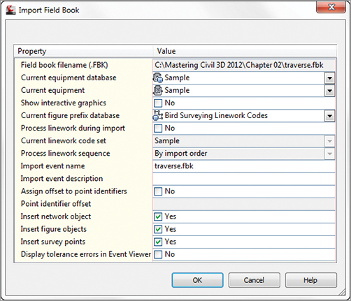
9. Right-click the Traverse Practice network and select Import Import Field Book.
10. Select the file traverse.fbk, which you can download from this book’s webpage (www.sybex.com/go/masteringcivil3d2012) and click Open. The Import Field Book dialog opens.
11. Make sure you have checked the boxes shown in Figure 2-14. You will be inserting the points into the drawing this time.
Figure 2-14: The Import Field Book dialog
12. Click OK. Save the drawing for the next exercise.
Inspect the data contained within the network. You have one control point—point 2—that was manually entered into the data collector. There is one direction, and there are four setups. Each setup combines to form a closed polygonal shape that defines the traverse. Notice that there is no traverse definition. In the following exercise, you’ll create that traverse definition for analysis:
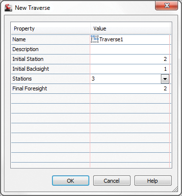
1. Continue working in the drawing from the previous exercise. Right-click Traverses under the Traverse Practice network and select New to open the New Traverse dialog.
2. Name the new traverse Traverse1.
3. Enter 2 as the value for the Initial Station and 1 (if necessary) for the Initial Backsight.
The traverse will now pick up the rest of the stations in the traverse and enter them in the next box.
4. Enter 2 as the value for the Final Foresight if necessary (the closing point for the traverse). Your New Traverse dialog box will look like Figure 2-15. Click OK.
Figure 2-15: Defining a new traverse
5. Right-click Traverse1 in the bottom portion of Toolspace. Select Traverse Analysis.
6. In the Traverse Analysis dialog, ensure that Yes is selected for Do Traverse Analysis and Do Angle Balance.
7. Select Least Squares for both the horizontal and vertical adjustment methods.
8. Select 30,000 for both the horizontal and vertical closure limit 1:X.
9. Leave Angle Error Per Set at the default.
10. Make sure the option Update Survey Database is set to Yes.
11. The Traverse Analysis dialog will look like Figure 2-16. Click OK.
Figure 2-16: Specify the adjustment method and closure limits in the Traverse Analysis dialog.

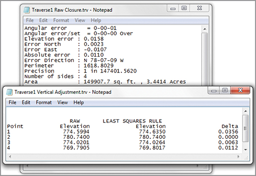
The analysis is performed, and four text files are displayed that show the results of the adjustment. Note that if you look back at your survey network, all points are now control points, because the analysis has upgraded all the points to control point status.
Figure 2-17 shows the Traverse1 Raw Closure.trv and Traverse 1 Vertical Adjustment.trv files that are generated from the analysis. The raw closure file shows that your new precision is well within the tolerances set in step 8. The vertical adjustment file describes how the elevations have been affected by the procedure.
Figure 2-17: Traverse analysis results
The third text file is shown in three separate portions. The first portion is shown in Figure 2-18. This portion of the file displays the various observations along with their initial measurements, standard deviations, adjusted values, and residuals. You can view other statistical data at the beginning of the file.
Figure 2-18: Statistical and observation data
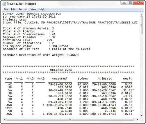
Figure 2-19 shows the second portion of this text file and displays the adjusted coordinates, the standard deviation of the adjusted coordinates, and information related to error ellipses displayed in the drawing. If the deviations are too high for your acceptable tolerances, you will need to redo the work or edit the field book.
Figure 2-19: Adjusted coordinate information
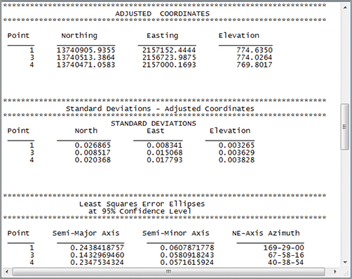
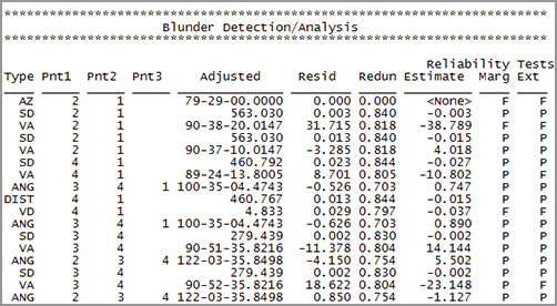
Figure 2-20 displays the final portion of this text file—Blunder Detection/Analysis. Civil 3D will look for and analyze data in the network that is obviously wrong and choose to keep it or throw it out of the analysis if it doesn’t meet your criteria. If a blunder (or bad shot) is detected, the program will not fix it. You will have to edit the data manually, whether by going out in the field and collecting the correct data or by editing the FBK file.
Figure 2-20: Blunder analysis
Other Methods of Manipulating Survey Data
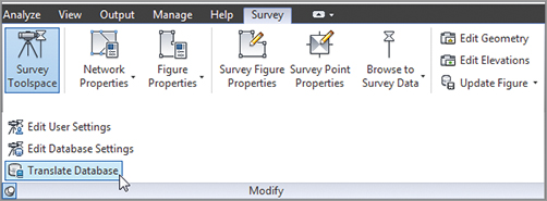
Often, it is necessary to edit the entire survey network at one time. For example, rotating a network to a known bearing or azimuth from an assumed one happens quite frequently. To find this hidden gem of functionality, change to the Modify tab and choose Survey from the Ground Data panel. Select the Survey tab, and choose Translate Database from the Modify panel (shown in Figure 2-21) to manipulate the location of a network.
Figure 2-21: The elusive yet indispensible Translate Database command
Manipulating the Network
Translating a survey network can move a network from an assumed coordinate system to a known coordinate system, it can rotate a network, and it can adjust a network from assumed elevations to a known datum.
1. Create a new drawing from the NCS Extended Imperial template file.
2. In the Survey tab of Toolspace, right-click and select New Local Survey Database. The New Local Survey Database dialog opens. Enter Translate in the text box. This is the name of the folder for the new database.
3. Click OK, and the Translate database will now be listed under the Survey Databases branch on the Survey tab.
4. Select Networks under the new Translate branch. Right-click and select New to open the New Network dialog. Enter Translate as the name of this new network. Click OK to dismiss the dialog.
5. Right-click the Translate network, and select Import Import Field Book.
6. Navigate to the file traverse.fbk which you can download from this book’s webpage, www.sybex.com/go/masteringcivil3d2012, and click Open. The Import Field Book dialog opens. Click OK to accept the default options.
7. Update the Point Groups collection in Prospector so that the points show up in the drawing if needed.
8. Draw a vertical polyline directly from point 3 (the point to the southwest), to the north of point 3 (toward the middle of the loop). It can be any length, but be sure to use the object snap node at point 3.
9. Change to the Modify tab and choose Survey from the Ground Data panel to open the Survey tab.
10. Choose Translate Database from the Modify panel drop-down menu.
11. For the purposes of this exercise, you will leave the points on their same coordinate system, but change the bearing of the line defined from point 3-point 2 to due north. Elevations will remain unchanged.
12. In the first window, type 3 as the Number value. This is the Base Point number (the number that you will be rotating the points around). Click Next.
13. In the next window, click the Pick In Drawing button in the lower-left corner to specify the new angle.
14. Using osnaps, pick point 3 and then point 2 (to the northwest) for your reference angle.
15. When you see the prompt Specify New Direction, pick point 3; somewhere along the orthogonal polyline you’ll be prompted to specify the second point to define the new angle, and pick point 3 again. Click Next.
16. In the next window, click the Pick In Drawing button on the lower left to pick point 3 as the destination point. This will essentially negate any translation features and provide you with only a rotation.
17. Leave the Elevation Change box empty. If you were raising or lowering the elevations of the network, this box is where you would enter the change value.
18. Click Next to review your results, and click Finish to complete the translation.
19. Go back to the drawing and inspect your points. Point 2 should now be due north of point 3.
20. Close the drawing without saving. Even though you did not save the drawing, the changes were made directly to the database and the network can be imported into any drawing.
Once figures are part of your drawing, you may have some cleanup to do. To edit a figure, select any one and use the commands from the context Ribbon that appears.
Be aware that reimporting your linework will result in your edits getting blown away. Reprocessing your linework after a modification is made can sometimes result in duplicate figures.
Using a Dirty Word, “Explode”
Most of the time in Civil 3D, exploding objects is a huge no-no. Exploding an object removes the underlying Civil 3D intelligence and reduces objects to base AutoCAD components. In this author’s opinion, survey figures are the exception to the no-exploding rule. An exploded survey figure will revert to a 3D polyline and will become divorced from the survey database that created it. Creating an independent polyline can be useful if your survey figures are going to be the basis for grading feature lines at a later time.
Other Survey Features
Other components of the survey functionality included with Civil 3D 2012 are the Astronomic Direction Calculator, the Geodetic Calculator, Mapcheck reports, and Coordinate Geometry Editor. All of these features are accessed from the Survey flyout on the Ground Data panel of the Analyze tab.
The Astronomic Direction Calculator, shown in Figure 2-22, is used to calculate sun shots or star shots. For the obscure art of these type of observations, Civil 3D has all the ephemeris data built in, making this a very convenient tool.
Figure 2-22: The Astronomic Direction Calculator

The Geodetic Calculator is used to calculate and display the latitude and longitude of a selected point, as well as its local and grid coordinates. It can also be used to calculate unknown points. If you know the grid coordinates, the local coordinates, or the latitude and longitude of a point, you can enter it in the Geodetic Calculator and create a point at that location. Note that the Geodetic Calculator only works if a coordinate system is assigned to the drawing in the Drawing Settings dialog. In addition, any transformation settings specified in this dialog will be reflected in the Geodetic Calculator, shown in Figure 2-23.
Figure 2-23: The Geodetic Calculator

Remember those labels you added to your lines in Chapter 1? Put them to work in a Mapcheck Report. The Mapcheck Report computes closure based on line, curve, or parcel segment labels.
1. Open the Mapcheck-start.dwg file, which you can download from this book’s webpage, www.sybex.com/go/masteringcivil3d2012.
2. Change to the Analyze tab, and select Survey Mapcheck from the Ground Data panel to display the Mapcheck Analysis palette.
3. Click the New Mapcheck button at the top of the menu bar.
4. At the Enter name of mapcheck: prompt, type Record Deed.
5. At the Specify point of beginning (POB) prompt, choose the north endpoint of the line representing the east line of the parcel (the longest line in the file).
6. Working clockwise, select each parcel label one at a time. Be sure not to skip the small segment in the southwest portion of the site.
7. In the northwest portion of the site, you will encounter a label whose bearing is flipped. You will use the Mapcheck Reverse command to rectify this in your mapcheck.
8. At the Select a label or [Clear/Flip/New/Reverse] prompt, type R and then press ↵ to reverse direction. The mapcheck glyph will now appear in the correct location along the segment, as shown in Figure 2-24.
Figure 2-24: The Mapcheck glyph verifies your input is correct.

9. Select the last line label along the north of the parcel.
10. Press ↵ to complete the mapcheck entry. The completed parcel should have 12 sides.
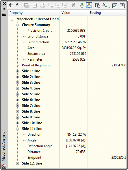
11. Select the output view as shown in Figure 2-25 to verify closure.
Figure 2-25: The completed deed in the Mapcheck Analysis palette
The Coordinate Geometry Editor
The new Coordinate Geometry Editor (Figure 2-26) is a powerhouse tool that makes creating and evaluating 2D boundaries easier than before. The functionality introduced with this feature supplants entering parcel data one segment at a time using the Line By Bearing And Distance command. Traverse analysis can be performed on manually entered segments, polylines, or COGO point objects without needing to define them in a survey database.
Figure 2-26: Your new best friend, the Coordinate Geometry Editor

Boundary data can be entered into the Coordinate Geometry Editor using a mix of methods. As shown in the first line of the traverse seen in Figure 2-26, you can use formulas to enter data. In the example shown, multiple segments with the same bearing have been consolidated into a single entry.
If a value is unknown, such as the distance in line 6 of Figure 2-26, you can enter a U. Civil 3D will calculate the unknown value when you generate the traverse report.
To enter data using points, use the Pick COGO Points In Drawing button to select the points in the direction of the traverse side. Note that the direction and distance are entered independently of each other, so you will need to repeat the selection for each column of the table. You may also copy and paste between columns.
If a line has been entered in error, the Coordinate Geometry Editor offers a variety of tools for fixing problems. To remove a line of the table, highlight the row, right-click, and select Delete Row, as shown in Figure 2-27.
Figure 2-27: Removing unwanted traverse data

Similar to the glyphs you saw in the Mapcheck command, the Coordinate Geometry will appear in the graphic showing the side directions and point of closure, as seen in Figure 2-28.
Figure 2-28: Temporary graphics or “glyphs” to help you identify your boundary

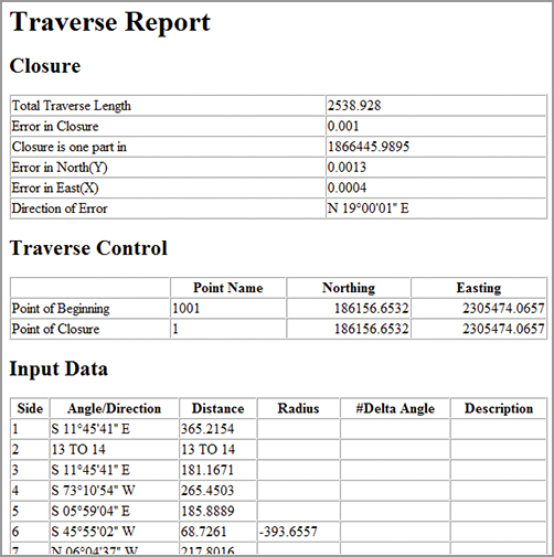
When you want to run a traverse report, set the report type you wish to run from the top of the Coordinate Geometry Editor. If you have unknowns in your traverse, your only option will be to calculate the unknown values. Click the Display Report button to view the results of your entries. Depending on the type of adjustment you chose, your results should resemble Figure 2-29.
Figure 2-29: Traverse report created by the Coordinate Geometry Editor