Now that you are familiar with the basics of object styles and label styles, you are ready to take your skills to the next level. The styles in the following section combine aspects of object styles and label styles.
You have a great deal of control over every detail, even ones that may seem trivial. Instead of being bogged down trying to understand every option, don’t be afraid to try a “trial and error” approach. If you make a change you don’t like, you can always edit the style until you get it right.
Table Styles
Civil 3D does a beautiful job of placing dynamically linked data tables that relate to your objects. The tables use the Text Component Editor to grab dynamic information from your objects. You also have control over fill colors, table headings, and how the data is sorted.
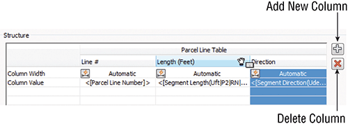
For the table style, the Data Properties tab contains all the column information. You can add columns by clicking the plus sign. You can remove columns by highlighting the column you want to remove and clicking the Delete button. Change column order by dragging them around and dropping them where you want them to go, as shown in Figure 19-104.
Figure 19-104: Modifying table columns
In the following exercise you will see the basic steps of modifying a table style. Now that you understand the ins and outs of the Label Style Composer, this procedure should be a breeze:
1. Open the Tables.dwg file. This file contains a parcel line table whose style you will modify.
2. Zoom into the parcel line table.
Notice there are several things you will want to change. The line numbers are out of order, the directions have far too much precision, and the length does not display units. All that is about to change.
3. Click the table to select it. From the context tab, select Table Properties Edit Table Style.
4. Switch to the Data Properties tab.
The Data Properties tab (Figure 19-105) is the main control area for all table styles. This is where you set behavior, text styles, and sizes for fields.
Figure 19-105: Data Properties tab for table styles

5. Place a check mark next to Sort Data. Set the sorting column to 1. Column 1 corresponds to the Column Value containing the Parcel Line Number. Set the order option to Ascending. The Ascending option will ensure that the parcel numbers are listed in the table from the lowest to highest value.
6. Double-click the column heading field for Length. Doing so opens a stripped-down version of the Text Component Editor. Headings and table titles are static text only; therefore only the text formatting tools are shown. Add (Feet) after the column heading to add a proper units heading to the column, as shown in Figure 19-106. Click OK.
Figure 19-106: Adding static text to a table column heading

7. Double-click the Direction Column value field. Doing so opens the Text Component Editor, similar to what you’ve used in earlier exercises. Click on the text in the preview area so that it becomes highlighted. Change Precision to 1 Second. Click the arrow to update the text. Click OK.
8. Click OK to complete the table style modifications.
Profile View Styles
When you are looking at a profile view that contains data, you are seeing many styles in play. The profiles themselves (existing and proposed) have a profile object style applied to them. The labeling has several styles applied to it, as you learned earlier in this chapter. Additionally, you will see profile view styles and band styles in action.
This section focuses on the profile view. A profile view controls many aspects of the display. The profile view style has a large role in determining:
- Vertical exaggeration
- Grid spacing
- Elevation annotation
- Title annotation
Figure 19-107 shows the basic anatomy of the profile view you have been working with throughout this book.
Figure 19-107: Profile view style and basic anatomy

In the example that follows, you will be making major modifications to a profile view style. The profile view that you will be practicing with does not contain any bands. Later on in this section, you will learn the ins and outs of band creation and modification.
1. Open the Profile View Styles.dwg file. This file contains a profile view with a very ugly style applied to it. You will be performing a complete makeover on this style.
2. Select the profile view by clicking anywhere on a grid line or axis. From the context tab, select Profile View Properties Profile View Style, as shown in Figure 19-108.
Figure 19-108: Accessing the profile view style

Position the dialogs on your screen so you can make changes to the style and observe the changes in the profile view behind it.
3. On the Graph tab, change the Vertical exaggeration to 10, as shown in Figure 19-109. Click Apply. If you can see your profile view in the background, you may be alarmed at the change. Don’t worry—you are not even close to done!
Figure 19-109: Change vertical exaggeration in the Graph tab of the Profile View Style dialog.

4. Switch to the Grid tab. Uncheck both Clip Vertical Grid and Clip Horizontal Grid options. Click Apply to observe the change. The vertical and horizontal grid lines will now extend to the entire length of the axes.
5. Change Grid Padding to 0.5 for Above Maximum Elevation and 0.5 for Below Datum. This setting will create additional space above and below the design data at least 0.5 times the vertical major tick interval (you will set the major tick interval later on). Click Apply to examine your changes.
6. Set all values for Axis offset to 0. This will ensure that the axes and the grid lines coincide around the edges of the view. Click Apply to examine your changes. The settings on the grid tab should now match what is shown in Figure 19-110.
Figure 19-110: The Grid tab: so many options!

7. Switch to the Title Annotation tab. You will be working on the left side of this dialog only. Change the Text height to 0.4″.
8. Click the Edit Text icon. In the Text Component Editor, remove all the text in the preview area. We will be starting over with a blank Text Component Editor.
From the Properties menu, select Parent Alignment and make these changes:
- Set Capitalization to Upper Case.
- Click the arrow to add the text to the preview.
- After the dynamic text, add a space and type PROFILE.
- Click OK to dismiss the Text Component Editor.
9. Change the Y offset for the title position to 0.5. Click Apply to examine your changes. If you do not see the changes, click OK and return to the dialog per Step 2. The Title Annotation tab should now match the settings shown in Figure 19-111.
Figure 19-111: Working with the graph view title size and placement

You will not bother to adjust any settings for the Axis title text on the right side of Figure 19-111 because the display will be turned off for all four of these possible elements.
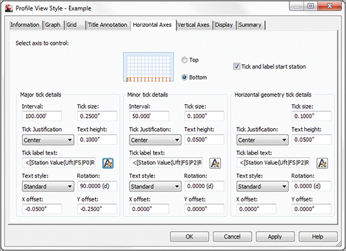
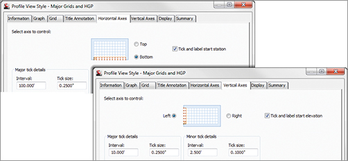
10. Switch to the Horizontal Axes tab. Make sure the Axis To Control radio button is set to Bottom.
11. Under Major Tick Details, set Interval to 100′.
12. For Tick Label Text, click the Edit Text icon. Highlight the dynamic station text that already exists in the preview by clicking it. Change the precision to 1. Click the arrow to update the text. Click OK to exit the Text Component Editor.
13. Still under Major Tick Details, change Rotation to 90. Change the X offset to –0.05″ and the Y offset to –0.25″.
14. Under Minor Tick Details, set Interval to 50′. No other changes are needed in the Minor Tick Details area. Click Apply to examine your changes. The Horizontal Axes tab should match the settings shown in Figure 19-112.
Figure 19-112: The bottom axis controls grid spacing.
15. Switch to the Vertical Axes tab. With the Select Axis To Control radio button set to Left, click the Edit Text icon for the major tick. In the Text Component Editor:
- Highlight the dynamic Profile View Point Elevation text by clicking on it.
- Change Precision to 1.
- Click the arrow to update the text.
- Click OK to exit the Text Component Editor.
16. Click the right radio button on the Vertical Axes tab to make it active. Click the Edit Text icon for the major tick. In the Text Component Editor:
- Highlight the dynamic Profile View Point Elevation text by clicking on it.
- Change Precision to 1.
- Click the arrow to update the text.
- Click OK to exit the Text Component Editor.
17. Click Apply to examine your changes. Figure 19-113 shows the Vertical Axes tab as yours should look at this point in the exercise (the tab has been stretched out to show the Tick Label Text field contents).
Figure 19-113: Don’t forget to change the settings for both left and right axes in this tab.

18. Switch to the Display tab. For this illustration, you will not need to set the layers. Turn off the following components:
- Left Axis Title
- Left Axis Annotation Minor
- Left Axis Ticks Minor
- Right Axis Title
- Right Axis Annotation Minor
- Right Axis Ticks Minor
- Top Axis Title
- Top Axis Annotation Major
- Top Axis Annotation Minor
- Top Axis Ticks Major
- Top Axis Ticks Minor
- Bottom Axis Title
- Bottom Axis Annotation Minor
- Grid At Horizontal Geometry Point
- Top Axis Annotation Horizontal Geometry
- Top Axis Ticks Horizontal Geometry
- Bottom Axis Annotation Horizontal Geometry
- Bottom Axis Ticks Horizontal Geometry
- Grid At Sample Line Stations
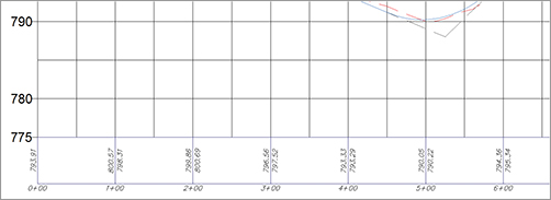
19. Click OK to complete the profile view style. Your profile view should resemble Figure 19-114.
Figure 19-114: Profile view after the style is completed
What Drives Profile View Grid Spacing?
On the Horizontal Axes tab and Vertical Axes tab of the Profile View Style dialog you may notice that you can control opposing axes separately. Each tab has a toggle for Select Axis To Control; Top or Bottom and Left or Right.
It is the Bottom and Left options in the respective tabs that control grid spacing. For both axes, you will find options for Major Tick Details. The Interval values for the major ticks are the key to getting the grid spacing to look the way you want. Changes to either horizontal or vertical major tick intervals will affect the height and length of the Profile view, as well as grid spacing. Changing the Interval on Minor Tick Details will affect the grid spacing, but will not affect the aspect ratio of the profile view.
A good rule of thumb is to set your bottom horizontal major tick Interval value equal to the view’s Vertical Exaggeration multiplied by the left vertical axis Interval value. For example, if you set the Vertical Exaggeration for the view to 10 on the Graph tab and your left vertical axis major tick Interval is 10′, the horizontal major tick Interval would be 100′.
Even if you don’t turn on the ticks or gridlines on these axes, the spacing increment will be reflected in the profile view.
Profile View Bands
Data bands are horizontal elements that display additional information about the profile or alignment that is referenced in a profile view. The most common band type is the profile data band. The other band types are not frequently used but can be helpful to designers by showing schematic representations of design as it relates to the profile stationing.
Bands can be applied to both the top and bottom of a profile view, and there are six band types:
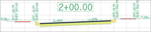
Profile Data Bands Display information about the selected profile. This information can include simple elements such as elevation, or more complicated information such as the cut-fill between two profiles at the given station. Figure 19-115 shows a typical profile data band.
Figure 19-115: Profile data band showing existing and proposed elevation in addition to major stations
Vertical Geometry Bands Create an iconic view of the elements making up a profile. Typically used in reference to a design profile, vertical data bands make it easy for a designer to see where vertical curves are located along the alignment. Figure 19-116 shows a typical vertical geometry data band.
Figure 19-116: Vertical geometry schematic shown in band
Horizontal Geometry Bands Create a simplified view of the horizontal alignment elements, giving the designer or reviewer information about line, curve, and spiral segments and their relative location to the profile data being displayed. Figure 19-117 shows a typical horizontal schematic data band.
Figure 19-117: Horizontal geometry shown as schematic in a data band
Superelevation Bands Display the various options for Superelevation values at the critical points along the alignment. Figure 19-118 shows an example of a superelevation data band.
Figure 19-118: Superelevation data in band form
Sectional Data Bands Displays information about the sample line locations, the distance between them, and other sectional-related information. In Figure 19-119 you can see a section data band showing sample line data.
Figure 19-119: Section data shown in a band
Pipe Data Bands Shows specific information about each pipe or structure being shown in the profile view. Figure 19-120 shows pipe data band with slopes and invert elevations.
Figure 19-120: Pipe data invert elevations and slope schematic in a band
Bands can be saved in band sets. Like alignment label sets and profile label sets, a band set determines which bands are applied to a profile view and will dictate the placement. The most common use for a band set is to create a single, viewable band and an additional nonvisible band for spacing purposes in plan and profile sheet generation.
In the following exercise, you will create a band that contains existing and proposed profile elevations:
1. Open the Profile Bands.dwg file. This file contains the profile view from the previous exercise and an empty band on the bottom of the view. You will be adding information to the profile data band.
2. From the Settings tab of Toolspace, select Profile View Band Styles Profile Data. Right-click the style called Example and select Edit.
3. On the Band Details tab, change Band Height to 1.0″.
4. On the right side of the Band Details tab, highlight Major Station and click the Compose Label button, as shown in Figure 19-121.
Figure 19-121: Band Details tab

5. On the Layout tab, click Add New Text Component:
- Change the name to Station.
- Change Anchor Point to Band bottom.
- Change Attachment to Top Center.
- Change the Y offset to –0.02″.
- Enter the Text Component Editor by clicking on the field that currently reads Label Text. Click the ellipsis.
- In the Text Component Editor, remove Label Text and select Station Value from the Properties list.
- Set Precision to 1.
- Click the arrow to add the dynamic text to the Preview window.
- Click OK to exit the Text Component Editor.
6. Click Add New Text Component again and make these changes:
- Change the name to Existing El.
- Change Anchor Point to Band Middle.
- Set the rotation angle to 90.
- Change Attachment to Bottom Center.
- Change the X offset to –0.02″.
- Enter the Text Component Editor by clicking on the field that currently reads Label Text. Click the ellipsis.
- In the Text Component Editor, remove Label Text and select Profile 1 Elevation from the Properties list.
- Verify the Precision is 0.01.
- Click the arrow to add the dynamic text to the preview window.
- Click OK to exit the Text Component Editor.
7. Click the Copy Text Component button and make these changes:
- Change the name to Proposed El.
- Change Attachment to Top Center.
- Set the X offset to 0.02″. Enter the Text Component Editor by clicking on the field that currently contains Profile 1 dynamic text. Click the ellipsis.
- In the Text Component Editor, remove the Profile 1 text and select Profile 2 Elevation from the Properties list.
- Verify the Precision is 0.01.
- Click the arrow to add the dynamic text to the preview window.
- Click OK to exit the Text Component Editor.
8. Click OK to finish working with the Major Stations and return to the Band Details tab.
9. Switch to the Display tab. Locate the Minor Tick component and turn it off.
10. Click OK. Select the profile and select Profile View Properties from the context tab.
11. On the Bands tab, scroll over until you see the column for Profile 2. Set the value for Profile 2 to Cabernet Court FG. Click OK. The completed band should resemble Figure 19-122.
Figure 19-122: Text along the bottom of your profile view in the form of a band
Section View Styles
Section view styles share many of the same concepts as creating Profile view styles. In fact, the Section View Style dialog has all the same tabs and looks nearly identical to the Profile View style.
In this section, you will walk through the creation of a section view style suitable for creating a section sheet:
1. Open the Section Styles.dwg file. This file contains section views created with the default settings for section views.
2. From the Settings tab of Toolspace, select Section View Section View Style Road Section. Right-click on Road Section and select Edit.
3. On the Grid tab, set the Grid padding settings to 0 for the Above Maximum Elevation and Below Datum options.
4. On the Display tab, turn off all components except:
- Graph Title
- Left Axis Annotation Major
- Right Axis Annotation Major
- Bottom Axis Annotation Major
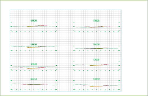
5. Click OK. Your section views should resemble Figure 19-123.
Figure 19-123: Yes, this is correct! A very stripped-down section view.

6. Select one of the views by clicking on the station label. From the context tab, select Update Group Layout. The section views will rearrange to fit up to six per page.
Why the bare-bones section view? The section view grid will come from the group plot style, so the only information we really need is in this simple style.
Group Plot Styles
The driver behind how section sheets get laid out on a page is the group plot style. Upon section creation, the group plot style takes the Section template file and fits sections inside the paperspace viewport:
1. Continue working in the Section Styles.dwg file. (If you did not successfully complete the previous exercise, you can start with Section Styles-2.dwg.) This file contains section views created with the default settings.
2. From the Settings tab of Toolspace, select Section View Group Plot Styles. Right-click on Basic and select Edit.
3. On the Array tab, change the column spacing to 4″. Change the row spacing to 2″, as shown in Figure 19-124.
Figure 19-124: The Array tab controls section view spacing
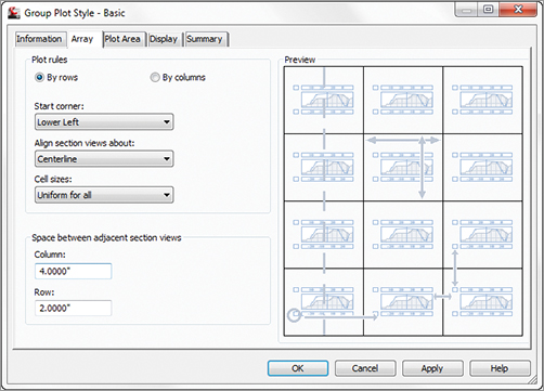
These spacing changes will allow more cross sections per page and additional room for scooting the views up and right to fit on the page better in the upcoming steps.
4. Switch to the Plot Area tab for observation purposes. Leave all the settings as shown in Figure 19-125. This is where the grid spacing we will be using on our sheets comes from.
Figure 19-125: The Plot Area tab is where grid spacing on sheets comes from.

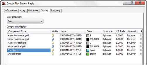
5. Switch to the Display tab. Under Component Display, turn on Major Horizontal Grid and the Major Vertical Grid. The components Minor Horizontal Grid and Minor Vertical Grid should be turned off. Set Color for the major grids to 9. Set Print Area to Cyan and Sheet Border to Green. Your Display tab will look like Figure 19-126.
Figure 19-126: Group plot style display components
6. Click OK to complete the group plot style edits.
Your section view sheets should be shaping up to the point where you could almost generate sheets. However, there is some text oozing out of the cyan line that represents the viewport border. In the next steps you will use a nonvisible section band to push the views onto the page.
7. Select any section view by clicking on the station label or the elevation labels. Select View Group Properties from the context tab. Click the ellipsis in the Change Band Set column, as shown in Figure 19-127.
Figure 19-127: Changing the band set in use for all section views

8. Verify the band type is set to Section Data. Set the band style as _NO DISPLAY. Click Add. Set the Gap distance to 0, as shown in Figure 19-128. Click OK to dismiss the Section View Group Bands dialog, and click OK to exit the View Group Properties dialog.
Figure 19-128: Add the data band and set the gap to 0.

9. Click Update Group Layout. The views will reorganize and form only one column per page. Don’t worry—next you will edit the _NO DISPLAY band style to fix this.
10. From the Settings tab of Toolspace, choose Section View Band Styles Section Data. Right-click on _NO DISPLAY and select Edit.
11. On the Band Details tab, change the band height to 0.2″. Change the text box width to 0.2″. The tab will resemble Figure 19-129.
Figure 19-129: Setting the band box size as a spacer

Even though the band is not visible, Civil 3D still accounts for this spacing when placing the views on the sheet. In this step, you are using this to your advantage.
12. Click OK to finish modifying the Data Band style.
13. Click the Update Group Layout button one last time. The cross section sheets should look like Figure 19-130.
Figure 19-130: The completed exercise
Code Set Styles
Code set styles determine how your assembly design will appear. Code set styles are used in many places. A code set style is in play when you first create your assembly. One is used in corridor creation and in the section editor. The most apparent use of a code set style is in section views like those that you created in the previous exercise.
Code set styles are a collection of many other styles. In a code set style you will find:
- Links and link label styles
- Points, point label styles, and feature line styles
- Shapes and shape label styles
- Quantity takeoff pay items
- Render materials for visualization tasks
It is helpful in naming your code set style to have the name of the set reflect its use. Multiple code set styles are needed because of different applications of its use. When you are designing an assembly, you may want to see more labels than when you are getting ready to plot the assembly in a cross-section sheet. Labeling that is useful in a cross-section sheet may obstruct your view of the design when working with it in the corridor cross-section editor.
The hardest part of working with code set styles is figuring out the name of the link or point you wish to label. Luckily, it is unusual for users to label shapes, so you won’t need to worry about those. The names of each point or link can be found in the subassembly properties. Most of the links and points are logically named, but there’s no harm in a little trial and error if you are not sure.
Shapes
Shapes are the areas that define materials. Because it is not common for people to label these materials in a section view, you will not be experiencing these in an exercise.
One heads-up, however: Resist the temptation to use a hatch pattern on shapes where multiple cross section views will be created. Solid fills and no patterns are your best bet to avoid performance issues and the annoying “Hatch pattern is too dense” warning.
Links and Link Labels
You learned in Chapter 8, “Assemblies and Subassemblies,” that a link is the linear part of a subassembly. The object style for the link itself is very simple; just a single linear component. The label for a link is usually expressed as a percent grade or as a slope ratio.
In the following exercise, you will modify a code set style to apply link labels to an assembly.
1. Open the Code Set Styles1.dwg file. This file contains a corridor and cross-section views. Zoom into one of the cross section views so you can observe the changes as you apply them to the code set style.
2. From the Settings tab of Toolspace, choose General Code Set Styles. Right-click on All Codes and select Edit.
3. In the Link list, locate Pave. Click the Label Tag icon in the Label Style column, as shown in Figure 19-131.
Figure 19-131: Adding labels to the link codes in the code set style
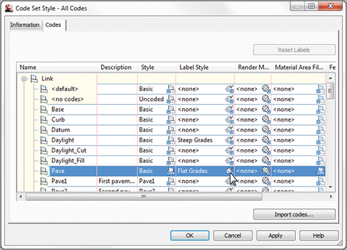
4. Select the Flat Grades label style and click OK. Click Apply to examine the change on the cross sections. You should see that the lanes now have slope information labeled.
5. In the Link list, locate Daylight. Click the Label Tag icon in the Label Style column and select Steep Grades as the label style. Click OK. Click OK to dismiss the All Codes label style and see what is happening with the cross section. The cross sections should resemble Figure 19-132.
Figure 19-132: Cross section with link labels applied to pave and daylight links

Points and Point Labels
A common frustration with new users of Civil 3D are the marker styles and their labels. For display in cross section views, you may not want points to display at all. In the following exercise, you will create a new code set style, modify point codes, and add more labels to the sections:
1. Continue working in the Code Set Styles1.dwg file or open Code Set Styles2.dwg.
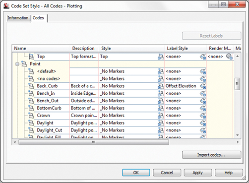
2. From the Settings tab of Toolspace, choose General Code Set Styles. Right-click on All Codes and select Copy.
3. On the Information tab, rename the style to All Codes-Plotting.
4. On the Codes tab, locate the Points category. Locate the Back_Curb point and click the Tag icon in the Label Style column. Set the style to Offset Elevation. Click OK.
5. Repeat step 4 to set the label style for Sidewalk_Out to Offset Elevation.
6. Click the first point name, <default>. While holding down the Shift key on your keyboard, scroll down to the last point listing, Top_Curb. With all of the points selected, click the Tag icon and change the style to _No Markers. The Code Set Style dialog should resemble Figure 19-133.
Figure 19-133: Points set to _No Markers and labels set to Offset-Elevation
7. Click OK. You do not see any changes to your cross sections yet because the style is not active.
8. Select a section view and select View Group Properties from the context tab.
9. Change the style of the corridor to the All Codes-Plotting style you created, as shown in Figure 19-134 and click OK.
Figure 19-134: Setting the code set style current on the section views

Your section view should now resemble Figure 19-135.
Figure 19-135: New code set style applied to the section view