A simple way to ensure that you’re referencing the specific data you want to reference is by assigning a name to the cell, or more typically to a range of cells, that you want to reference. For example, the WORKDAY function allows an argument providing specific non-work days, such as holidays. This is very convenient because not everyone celebrates the same holidays.
To simplify the process of creating formulas that refer to a specific range of data, and to make your formulas easier to read and create, you can refer to a cell or range of cells by a name that you define. For example, you might use the name Interest for a cell containing an interest rate, or you might use the name Holidays for a range of cells containing non-work days. In a formula, you refer to a named range by name. Thus you might end up with a formula like this:
=WORKDAY(StartDate,DaysOfWork,Holidays)
A formula using named ranges is simpler to understand than its standard equivalent, which could look like this:
=WORKDAY(B2,B$3,Data!B2:B16)
Referring to a named data range, rather than to a specific range of cells, is far simpler and also lessens the chance of error.
Tip
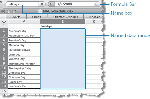
The range name is visible in the Name box at the left end of the Formula Bar, and in the various Names dialog boxes. If a cell is part of multiple named ranges, only the first name is shown in the Name box. The Name box displays the name of a multiple-cell named range only when all cells in the range are selected.
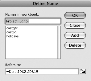
After defining a named range, you can change the range name or the cells included in the named range, or delete a range name definition, from the Define Name dialog box.
To define a selected cell or range of cells as a named range:
On the Insert menu, point to Name, and then click Define.
The Define Name dialog box opens. The content of the upper-left selected cell is displayed in the Names In Workbook box as a suggested range name. The selected cells are displayed in the Refers To box.
Verify or change the range name and cell range, and then click Add.