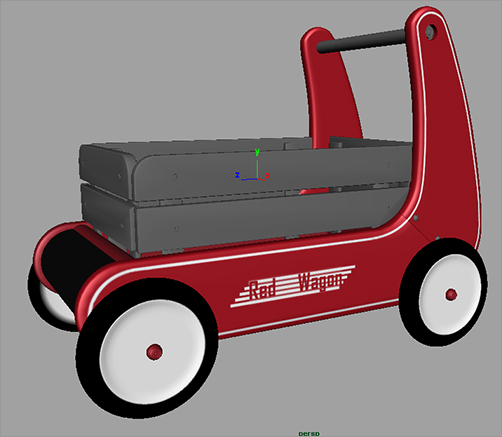
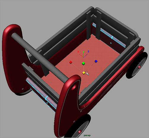
Figure 7-42: The red wagon
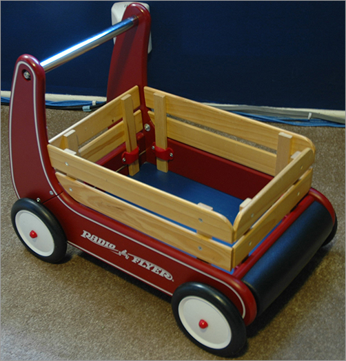
Using the wagon model from Chapter 6, you’ll now assign shaders to the red wagon shown in Figure 7-42. Take a good look at the image of the toy wagon in the Color Section of the book to see how the red wagon is colored. The wagon is fairly simple; it will need a few colored shaders (Red, Black, Blue, and White) for the body, along with a few texture maps for the decals—which is where the real fun begins. The wagon will also require some more intricate work on the shaders and textures for the wood railings and silver metal screws, bolts, and handlebar; these will be a good foray into image maps and UVs.
This exercise is a prime example of how lighting and shading go hand in hand.
Assigning Shaders
Load the file RedWagonModel_v08.ma from the Scenes folder of the RedWagon project to begin shading the finished model of the wagon.
Shading is the common term for adding shaders to an object.
Study the color images of the wagon, and see how light reflects off its plastic, metal, and wood surfaces. Blinn shaders will be perfect for nearly all the parts of the wagon. Follow these steps:
1. Open the Hypershade window, and create four Blinn shaders.
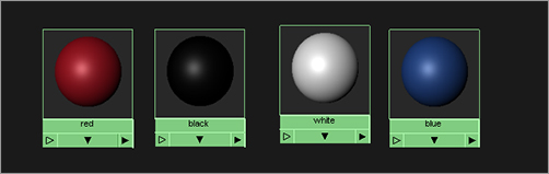
2. Assign the following HSV values to the Color attribute of each Blinn shader, and name them as shown in Table 7-1 and in Figure 7-43. You’ll create the Chrome Metal and Wood shaders later.
Figure 7-43: Create the four-colored Blinn shaders.
HSV Color Values for the Wagon’s Colors

Initial Assignments
Look at the photo of the wagon in the Color Section in the middle of this book. The bullnose and tires are black, the wheel rims are white, the floor is blue, the screws and bolts and handlebar are chrome metal, the railings are wood, and the main body is red. Assign shaders to the wagon according to the color photo and the following steps:
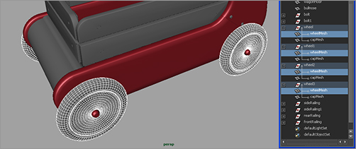
1. In the view panel, select the side panels (the A and B panels, without the screws and bolts) and the wheel rim caps, as shown in Figure 7-44, and assign the Red Blinn shader to them. Press 6 to enter into Texture Display mode.
2. Select the wheelMesh objects for all four wheels, and assign them the White shader. The tires also turn white, but you’ll fix that shortly; don’t worry about it now. See Figure 7-45.
Figure 7-44: Assign the Red shader.

Figure 7-45: Assign the White shader.
3. Select the bullnose (the rounded cylinder in front of the wagon), and assign it the Black Blinn.
4. Select the wagon floor object, and assign it the Red shader, as shown in Figure 7-46. You’ll notice that the front and back body of the wagon turn red as they’re supposed to, but so does the floor of the wagon, which should be blue according to the photo in the Color Section. If you try to assign the Blue shader to the wagon floor mesh, the floor will be correct, but the front and back body of the wagon will be blue and not red. You’ll fix this later.
Now you have initial assignments for the basic colors of the wagon’s body. Let’s tweak these shaders’ colors next.
Figure 7-46: Assign the Red shader to the wagon floor for now.

Creating a Shading Network for the Wheels
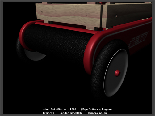
Figure 7-47: The tire on the wagon
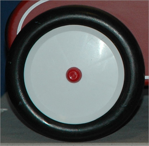
Refer to Figure 7-47 to observe how the materials are different between the rim and the tire for the wheels. The rim is glossier and has a tighter, sharper specular, whereas the tire has a very diffuse specular and is quite bumpy. As you did for the axe exercise, you’ll create a Layered shader for the wheels with white feeding into the rim portion and black into the tire.
Coloring the Wheel
First, you need to determine where the white ends and the black starts on the surface of the wheel mesh:
1. Select the White shader in the Hypershade window. Click the Map button (![]() ) next to the Color attribute. Make sure that Normal is checked. Click Ramp to create a Ramp texture. The wheel’s color turns to a red, green, blue gradient, but in the wrong direction; you need the gradient to run from the center to the edge and not clockwise across the wheel. In the Ramp texture’s Attribute Editor, set the Type to U Ramp, as shown in Figure 7-48.
) next to the Color attribute. Make sure that Normal is checked. Click Ramp to create a Ramp texture. The wheel’s color turns to a red, green, blue gradient, but in the wrong direction; you need the gradient to run from the center to the edge and not clockwise across the wheel. In the Ramp texture’s Attribute Editor, set the Type to U Ramp, as shown in Figure 7-48.
Figure 7-48: Set the ramp to a U Ramp type.

If the ramp doesn’t show up in your view panels, make sure you press 6 to enter Texture Display mode. If the colors and ramp texture still don’t display, make sure Use Default Material isn’t checked in the view panel’s Shading menu.
2. Now the color gradient is running from the center (red) to the outside edge (green) to blue on the reverse side of the wheel. Move the blue ramp’s handle in the ramp’s Attribute Editor until its Selected Position value is about 0.6, as shown in Figure 7-49.
3. Delete the red handle in the ramp by clicking the checked box on the right of the handle. Change the blue color to black and the green color to white. Set the Interpolation attribute (found above the ramp color) to None so you get clean transitions from white to black, instead of a soft linear gradient where the black slowly grades to white. Name this ramp wheelPositionRamp.
4. The backs of the wheels are solid black. In the wheelPositionRamp, click toward the top of the ramp to create a new color. Set that color to white, and set its position to about .920 to place white behind the wheels, keeping the black only where the tire is. See Figure 7-50.
Now that you’ve pinpointed where the white rim ends and the black tire begins, you’ll use this ramp as a transparency texture to place the Tire shader on top of the Rim shader in a Layered shader that you’ll create later.
Figure 7-49: Move the blue handle.

Figure 7-50: Setting the tire location using a ramp

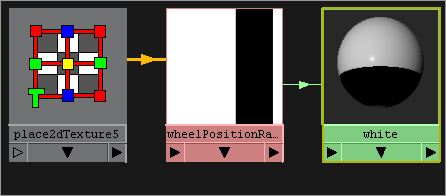
5. You don’t need this Ramp shader on the color of the shader anymore—you did this so you could easily see the ramp color positions in the view panels. In the Hypershade, select the White shader, and click the Input and Output Connections icon (![]() ) to graph the shader, as shown in Figure 7-51.
) to graph the shader, as shown in Figure 7-51.
Figure 7-51: The White shader has the ramp attached as color.
6. In the Attribute Editor, RMB+click the Color attribute, and select Break Connection from the context menu to disconnect the ramp from the color. Set the Color back to white. Notice that the link connecting the Ramp texture node to the White shader node disappears in the Hypershade window.
Figure 7-52: Drag the White shader to the Layered shader, and delete the default Green shader from it.
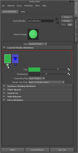
7. Create a Layered shader. MMB+drag the White shader from the Hypershade to the top of the Layered Shader Attributes window, as shown in Figure 7-52. Delete the default Green shader in the Attribute Editor by clicking the checked box below its swatch.
8. Create a new Blinn shader, and set its color to black. Name the shader tireShader. Select the Layered shader, and then MMB+drag the new tireShader from the Hypershade to the Layered shader’s Attribute Editor, placing it to the left of the White shader, as shown in Figure 7-53. Name the Layered shader wheelShader.
9. Select the wheels, and assign the wheelShader Layered shader to them. The wheels should appear all white. This is where the ramp you created earlier (wheelPositionRamp) comes into play.
10. Select the wheelShader, and click Input and Output Connections to graph the network in the Work Area of the Hypershade window. In the top panel of the Hypershade, click the Texture tab to display the texture nodes in the scene, so you can see wheelPositionRamp’s node.
Figure 7-53: Add the black tireShader.
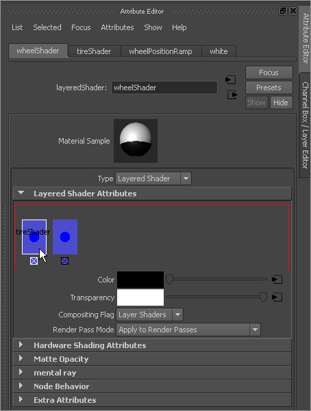
11. In the wheelShader’s Attribute Editor, click the tireShader swatch on the left. MMB+drag the wheelPositionRamp node to the Transparency attribute, as shown in Figure 7-54.
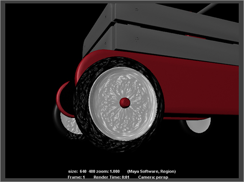
12. When you attach the ramp, the wheelShader icon turns white on top and black on the bottom. Render a frame in the persp panel to make sure the black tires line up properly, as shown in Figure 7-55. The wheel coloring is complete!
Figure 7-54: Attach the ramp to the Transparency of the tireShader in the wheelShader.
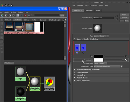
Figure 7-55: The tires are done!

Hey, Hold on a Minute…
Why did you go through a Layered shader with two different shaders (one white and one black) when you could more easily use one shader and assign the same black to white ramp to its color? Because the white rim and the black tire are different materials, and you need to use two different shaders to properly show that in renders.
Setting the Feel for the Materials and Adding a Bump Map
Because the material look and feel on the real wheels differs quite a bit between the rim and the tire, you’ll further tweak the white rim and the black tire shaders. The rim is a smooth, glossy white, and the tire is a bumpy black with a broad specular. Follow these steps:
Figure 7-56: Set your view to this angle, and render a frame.

1. Let’s set up a good angle of view for your test renders. Position your persp view to resemble the view in Figure 7-56. Render a frame.
2. Select the White shader, and set Eccentricity to 0.05 and Specular Roll Off to 0.5. Doing so sharpens the specular highlight on the rim.
3. Select the black tireShader, and set Eccentricity to 0.375 and Specular Roll Off to 0.6 to make the highlight more diffuse across the tire. Set Reflectivity to 0.05. Render a frame, and refer to Figure 7-57 to see how the specular highlight is broader and less glossy than in Figure 7-56.
Figure 7-57: Setting specular levels

Figure 7-58: The whole wheel becomes bumpy!
4. Open the Attribute Editor for the tireShader, and click the Map icon (![]() ) next to the Bump Mapping attribute. In the Create Render Node window, click to create a Fractal texture map. Notice that the entire wheelShader icon becomes bumpy. Render a frame, and you’ll see that the entire wheel is bumpy—not just the tire. (See Figure 7-58.) Argh!
) next to the Bump Mapping attribute. In the Create Render Node window, click to create a Fractal texture map. Notice that the entire wheelShader icon becomes bumpy. Render a frame, and you’ll see that the entire wheel is bumpy—not just the tire. (See Figure 7-58.) Argh!
5. You have to use the wheelPositionRamp to prevent the bump from showing on the rim. Select the wheelShader, and click the Input and Output Connections icon (![]() ) in the Hypershade to graph its network (Figure 7-59).
) in the Hypershade to graph its network (Figure 7-59).
Figure 7-59: Graph the wheelShader network.

Notice the single, blue connecting line between the fractal1 node and the bump2d1 node in the Hypershade. This means the alpha channel of the fractal feeds the amount of bump that is rendered on the tireShader. You have to alter the alpha coming out of the fractal node with the positioning ramp to block the rim from having any bump. The white areas of the ramp allow an output in alpha from the fractal, which creates a bump for the surface; whereas the black area of the ramp keeps any bump from appearing. Because you already used this ramp to position the Rim shader and the Tire shader on the wheel, it will work perfectly for the bump position as well.
Figure 7-60: MMB+drag the ramp to the Alpha Gain of the fractal.
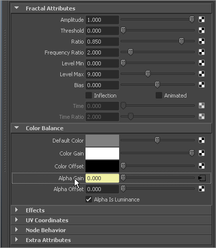
6. Select the fractal to display it in the Attribute Editor, and MMB+drag the wheelPositionRamp in the Hypershade to the Alpha Gain attribute for the fractal, as shown in Figure 7-60.
7. Render a frame, and you see that now the tire has no bump and the rim is bumpy (Figure 7-61).
8. This is easy enough to fix. All you need to do is reverse the ramp and then feed it into the Alpha Gain of the fractal so that the tire is bumpy and the rim is smooth. In the Hypershade, in the Create pane on the left, click the Maya ⇒ General Utilities heading, and then select the Reverse icon to create a reverse node in the Hypershade window. See Figure 7-62.
9. In the Hypershade, MMB+drag the wheelPositionRamp node onto the Reverse node, and select Input from the context menu when you release the mouse button. This connects the output of the ramp into the reverse node, which will then reverse the effect of the ramp on the fractal when you connect it in the next step.
Figure 7-61: The tire is smooth and now the rim is bumpy.

Figure 7-62: Create a reverse node.
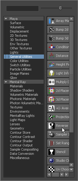
Figure 7-63: Connecting the reverse node to the fractal node
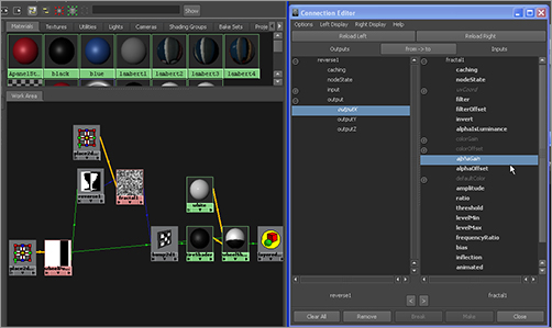
10. MMB+drag the reverse node on top of the fractal1 node, and select Other from the context menu. This opens the Connection Editor, which you first saw in Chapter 3. On the left is loaded the reverse1 node, and on the right is the fractal1 node. In the left pane, click the plus sign next to the Output attribute, and select output.X. In the right pane, select the alphaGain attribute, as shown in Figure 7-63.
11. Open the Render Settings window by choosing Window ⇒ Rendering Editors ⇒ Render Settings. Click the Maya Software tab, and set Quality to Production Quality in the pull-down menu. (See Figure 7-64.) Render a frame: you finally have a bump on the tire and a smooth rim. See Figure 7-65.
12. It’s not a very convincing bump yet, so select the fractal node and set Ratio to 0.85. Click the Placement tab for the fractal (it should be called something like place2dTexture6), and set the Repeat UV values to 18 and 48, as shown in Figure 7-66. Doing so makes the fractal pattern finely speckled on the tire.
13. Render a frame: the fractal’s scale on the bumpy tire looks too strong. Double-click the bump2d node in the Hypershade, and, in the Attribute Editor, set Bump Depth to 0.04. Render, and check your frame against Figure 7-67. The bump looks much better, if not a little strong from this angle; you can finesse it to taste from here.
Figure 7-64: Set Quality to Production Quality.
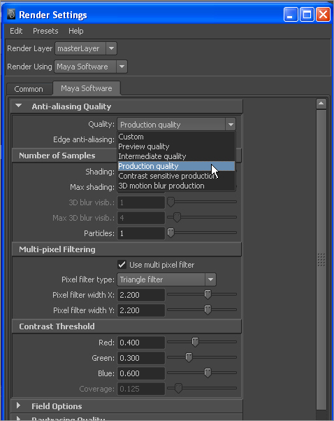
Figure 7-65: Now you’ve got the bump where you need it.

Figure 7-66: Set the Repeat UV values for the fractal map.
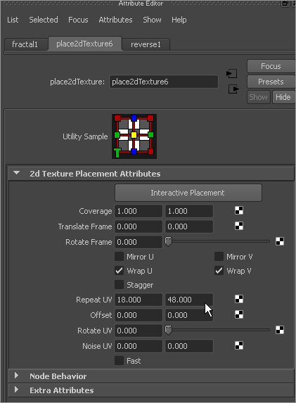
Figure 7-67: The wheel looks pretty good.

Tire Summary
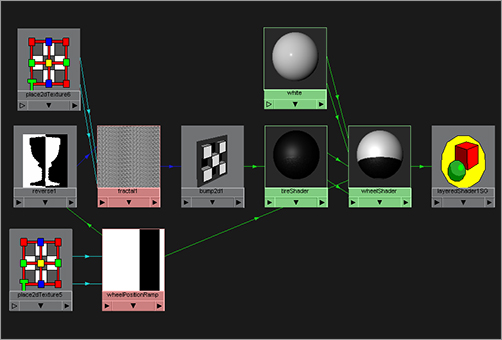
Congratulations! You’ve made your first somewhat complex shading network, as shown in Figure 7-68. By now, you should have a pretty good idea of how to get around the Hypershade and create shading networks. To recap, you’re using a ramp to place the two Tire and Rim shaders on the wheel, as well as using it to place the bump map on just the tire by using a reverse node. The more you make these shading networks, the easier they will become to create.
Figure 7-68: Your first complex shading network
This type of shading is called procedural shading, because you used nothing but stock Maya texture nodes to accomplish what you needed for the wheels. In the following sections, you’ll make good use of image mapping to create the decals for the wagon body as well as the wood for the railings.
You can load the file RedWagonTexture_v01.ma from the Scenes folder of the RedWagon project to check your work or skip to this point.
Putting Decals on the Body
Figure 7-69 shows you the decals that need to go onto the body of the wagon. They include the wagon’s logo, which you’ll replace with your own graphic design, and the white stripe that lines the side panels.
Instead of trying to make a procedural texture as you did with the wheel, you’ll create an image map that will texture the side panels’ white stripe. The stripe is far too difficult to create otherwise. You’ll create an image file using Photoshop (or other such image editor) to make sure the white stripe (and later the red wagon logo) lines up correctly.
Figure 7-69: You need to add the body decals.

Working with UVs
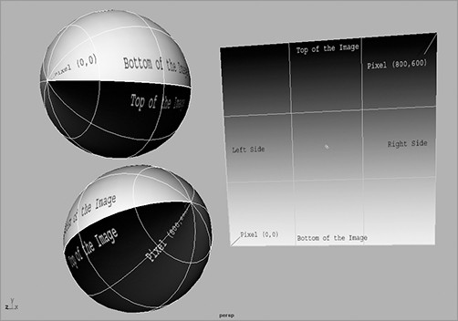
Mapping polygons can involve the task of defining UV coordinates for them so that you can more easily paint an image map for the mesh. When you create a NURBS surface, UV coordinates are inherent to the surface. At the origin (or the beginning) of the surface, the UV coordinate is (0,0). When the surface extends all the way to the left and all the way up, the UV coordinate is (1,1). When you paint an 800 × 600–pixel image in Photoshop, for example, it’s safe to assume that the first pixel of the image (at X = 0 and Y = 0 in Photoshop) will map directly to the UV coordinate (0,0) on the NURBS surface, whereas the topmost right-corner pixel in the image will map to the UV (1,1) of the surface. Toward that end, mapping an image to a NURBS surface is fairly straightforward. The bottom of the image will map to the bottom of the surface, the top to the top, and so on. Figure 7-70 shows how an image is mapped onto a NURBS plane and a NURBS sphere.
The locations in the image, marked by text, correspond to the positions on the NURBS plane. The sphere, because it’s a surface bent around spherically, shows that the origin of the UV coordinates is at the sphere’s pole on the left and that the image wraps itself around it (bowing out in the middle) to meet at the seam along the front edge as shown.
When you’re creating polygons, however, this isn’t always the case. You must sometimes create your own UV coordinates on a polygonal surface to get a clean layout on which to paint in Photoshop. Although poly UV mapping becomes fairly involved and complicated, it’s a concept that is important to grasp early. When poly models are created, they have UV coordinates; however, these coordinates may not be laid out in the best way for texture-image manipulation.
Figure 7-70: An image file is mapped to a NURBS plane and a NURBS sphere. Notice the locations marked in the image and how they map to the locations on the surface, with the pixel coordinates directly corresponding to the surface’s UV coordinates.
Working with the A Panels
This section assumes that you have some working knowledge of Adobe Photoshop. You can skip the creation of the maps and use the maps already on the CD, which are called out in the text later in the exercise.
First, let’s look at how the UVs are laid out for the A panel that you modeled in Chapter 6:
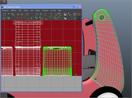
1. Using your scene or the scene file RedWagonTexture_v01.ma from the Scenes folder of the RedWagon project, select the A panel on one side of the wagon, and choose Window ⇒ UV Texture Editor, as shown in Figure 7-71.
The UV Texture window works almost like any other view panel. You may navigate the window and zoom in and out using the familiar Alt + mouse button combinations.
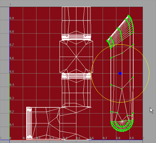
2. RMB+click any part of the wireframe layout in the UV Texture Editor window, and select UV to enter the UV selection. Select the entire wireframe mesh at lower right, as shown in Figure 7-72. Notice that green points are selected—almost as if they were vertices. These are UV points, and they’re what define the UV coordinates on that part of the mesh. Look in the Perspective view panel; the entire front face of the A panel is selected as well the green UV points (also in Figure 7-72).
Figure 7-71: The A Panel in the UV Texture Editor

Figure 7-72: Select the UVs on this part of the A panel mesh.
Feel free to select parts of the UV layout in the UV Texture Editor to see what corresponding points appear on the mesh in the persp panel. This will help orient you as to how the UV layout works on this mesh.
Figure 7-73: Convert the UVs you just selected to a face selection. This method easily isolates the front faces of the A panel for you to lay out their UVs again.

3. You need to again lay out just this area of the mesh’s UVs. Because you already have the entire front side of the panel selected in UVs, let’s convert that selection to poly faces on the model. In the Polygons menu set and in the main Maya menu bar, choose Select ⇒ Convert Selection ⇒ To Faces. The front faces of the A panel mesh are selected, as shown in Figure 7-73. You can always manually select just the front faces of the mesh, but this conversion method is much faster. The UV Texture Editor shows just those faces now.
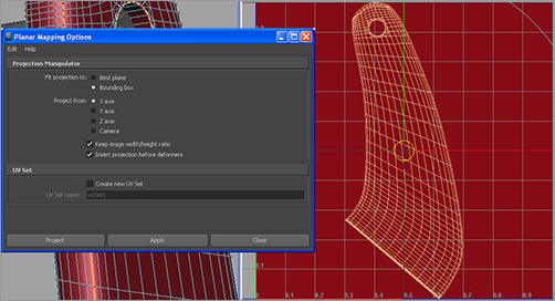
4. With those faces selected, make sure you’re in the Polygons menu set. Choose Create UVs ⇒ Planar Mapping ❒ from the Main Menu bar. In the option box, set the Project From option to X Axis, check the Keep Image Width/Height Ratio option, and then click Project. (See Figure 7-74.) The UV Texture Editor shows the front A panel face.
Figure 7-74: Create a planar projection for the UV layout.
5. Now the front face has a much simpler UV layout from which to paint. However, it’s centered in the UV Texture Editor and will overlap the other UVs of the same mesh. You should move and size it to fit into its original corner, more or less, to make sure no UVs double up on each other. In the UV Texture Editor, right-click the wireframe, and select UV to enter UV selection. Select all the UVs on those faces; all the UVs for the A panel mesh appear in the UV Texture Editor, and you can see the overlap. See Figure 7-75.
6. Press W for the Move tool, and move the selected UVs to the side of the UV Texture Editor. Press R for the Scale tool, and scale them down a bit to fit into the corner, as shown in Figure 7-76.
Figure 7-75: The UVs for the A panel, with the front side’s UVs still selected
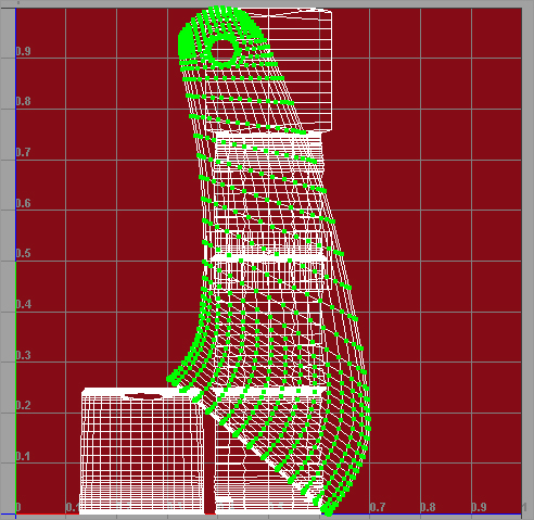
Figure 7-76: Position these UVs to make sure they don’t overlap the rest of the A panel mesh’s UVs.
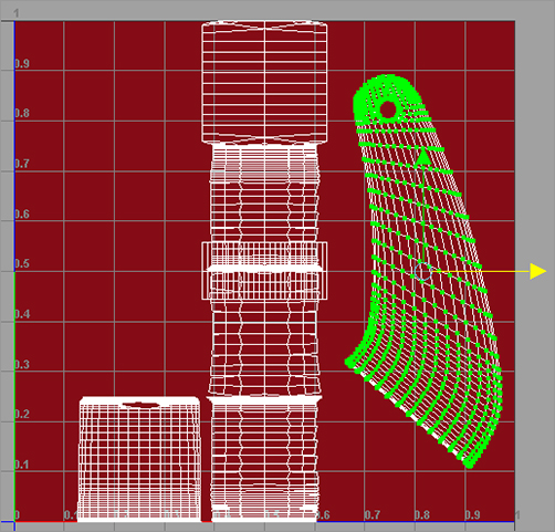
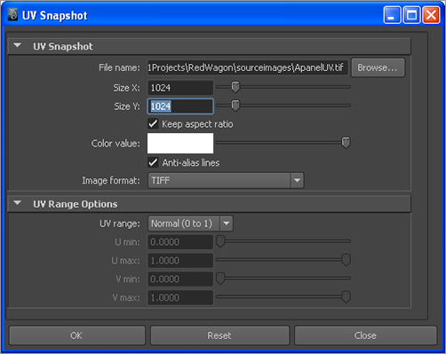
Figure 7-77: Settings for the UV snapshot
7. Earlier in the chapter, you saw how to write out a PSD file with a UV snapshot as one of its layers. You’ll use a similar technique to paint the decal for the panel. Click an empty area of the UV Texture Editor to deselect everything. Then, in Object Selection mode (press F8 if you need to exit Component Selection), select the A panel mesh in the persp panel.
8. In the UV Texture Editor window, select Polygons ⇒ UV Snapshot to open the Options window. Set both Size X and Size Y to 1024. Change the image format to TIFF, click the Browse button at the top next to the File Name field, and navigate to the RedWagon project’s Sourceimages folder on your hard drive. Name the file ApanelUV.tif, and click Save. Leave UV Range set to Normal (0 to 1), and click OK. See Figure 7-77.
Working in Photoshop
Next, you’ll go into Photoshop to paint your map according to the UV layout you just output:
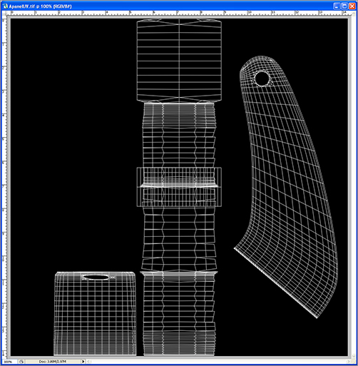
1. In your OS file browser, navigate to the RedWagon project’s Sourceimages folder, and open the file ApanelUV.tif in Photoshop. Figure 7-78 shows the layout of the UVs that you’ll use to create the white stripe for the front of the A panel.
Figure 7-78: Working with the UV layout for the A panel will be easy.
2. In Photoshop, create a new layer on top of the background layer that is the UV layout (white on black, as shown). Using the Bucket tool, fill that new layer with the same red you used on the shader in your scene. To do so, click the foreground color swatch in Photoshop, and set H to 355, S to 91 percent, and B to 65 percent, as shown in Figure 7-79. Click OK.
3. Using the Bucket tool, click to fill the entire image with the red you just created. The trouble is that now you can’t see the UV layout. Set the Opacity of the red layer in Photoshop to 50 percent, as shown Figure 7-80.
4. Set Photoshop’s foreground color to white. Using the Line and Brush tools set to a width of about 6 pixels, draw a stripe following the UV layout lines, as shown in Figure 7-81. Doing so places that white stripe along the A panel’s outer edge, because the UV lines you’re following correspond to that area of the mesh. The rest will be left red.
Figure 7-79: In Photoshop’s Color Picker, create the same red you used for the wagon.

Figure 7-80: Set the opacity for the red layer in Photoshop so you can see the UV layout on the layer below.

Figure 7-81: Follow the UV lines to draw the white stripe.

Figure 7-82: The striped image file
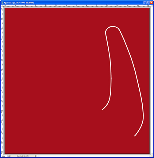
5. You may have drawn directly on the red layer in Photoshop or created a new layer for the stripe. In either case, set the Opacity of the red layer back to 100 percent so you can no longer see the UV layout. Your image file should look like the one in Figure 7-82. Save the image as ApanelStripe.tif in the Sourceimages folder of your RedWagon project. You may keep the layers in the TIFF file, or you may choose to flatten the image or merge the layers. It may be best to keep the stripe and red on separate layers so that you can go back into Photoshop and edit the stripe as needed.
Creating and Assigning the Shader
Now, let’s create the shader and get it assigned to the geometry:
1. Back in Maya, open the Hypershade, and select the Red shader. Duplicate it by choosing Edit ⇒ Duplicate ⇒ Shading Network in the Hypershade window, as shown in Figure 7-83.
Figure 7-83: Duplicate the original Red shader.

2. Name the new shader (called red1) ApanelStripe. Open the Attribute Editor, click the Map button (![]() ) next to Color, and choose File. In the Attribute Editor, click the Folder icon next to the Image Name field. Navigate to your Sourceimages folder, and select ApanelStrip.tif, as shown in Figure 7-84.
) next to Color, and choose File. In the Attribute Editor, click the Folder icon next to the Image Name field. Navigate to your Sourceimages folder, and select ApanelStrip.tif, as shown in Figure 7-84.
3. In the Hypershade, you may see that the Shader icon has turned somewhat transparent. Maya is automatically mapping the Transparency attribute of the shader as well as the color. Double-click the shader to open its Attribute Editor, RMB+click Transparency, and select Break Connection from the context window. Doing so sets the shader to the same red you used earlier, but now it gives you a stripe along the side A panel.
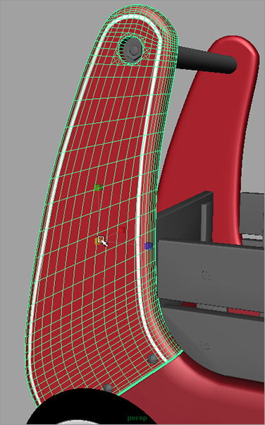
4. Assign the ApanelStripe shader to the A panel mesh, and press 6 for Texture Display mode in the persp panel. See Figure 7-85. The stripe lines up well.
You may skip the image creation using Photoshop and use the ApanelStripe.tif image file found in the Sourceimages folder of the RedWagon project on the CD instead.
Figure 7-84: Select the ApanelStripe.tif file.
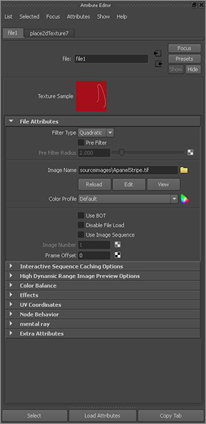
Figure 7-85: The stripe

Copying UVs
You need to put the stripe on the other side’s A panel. Select the other A panel, and assign the ApanelStripe shader to it. You’ll notice that no stripe appears. (See Figure 7-86.) This is because the UV layout for this A panel hasn’t been set up yet. Don’t worry; you don’t have to redo everything you did for the first A panel. You can essentially copy the UVs from the first A panel mesh to this one:
Figure 7-86: Assign the ApanelStripe shader to the other side’s A panel.

Figure 7-87: The Transfer Attributes settings

1. Select the first A panel (with the stripe) and the second panel (without the stripe). In the Polygons menu set, choose Mesh ⇒ Transfer Attributes ❒. In the option box, set Sample Space to Local, as shown in Figure 7-87, and click Transfer.
2. The stripe appears on the inside of the back A panel, and not on the outside as you need. Select that A panel, and choose Modify ⇒ Center Pivot.
3. In the Channel Box, enter a value of -1.0 for Scale X. The stripe flips to the correct side, as shown in Figure 7-88.
4. With that A panel still selected, choose Modify ⇒ Freeze Transformations.
You can load the file RedWagonTexture_v02.ma from the Scenes folder of the RedWagon project to check your work or skip to this point.
Figure 7-88: The stripe is on the correct side now.
The file texture you’ll use for the panels were painted in Photoshop to place the stripes and logo properly on the wagon using their UV layouts. Study the image file, and see how it fits on the mesh of the wagon. Try adjusting the image file with your own artwork to see how your image map affects the placement on the mesh.
Working with the B Panels
With the A panels done, you’ll move on to the B panels, using much the same methodology you did with the A panels. To begin, follow these steps:
1. Select one of the B panels, shown in Figure 7-89, and open the UV Texture Editor window.
2. As you did with the front face of the A panel, select the UVs on the lower-right side of the layout in the UV Texture Editor, as shown in Figure 7-90, to isolate the front face of the B panel.
3. Choose Select ⇒ Convert Selection ⇒ To Faces. You’ve isolated the front face of the B panel.
4. Choose Create UVs ⇒ Planar Mapping ❒. In the Options box, set the Project From option to X Axis, and make sure the Keep Image Width/Height Ratio option is checked, just as before. Your B plane shows up nicely laid out in the UV Texture Editor. See Figure 7-91.
Figure 7-89: Starting on the B panels
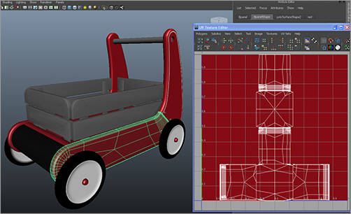
Figure 7-90: Select the front face UVs for the B panel.

Figure 7-91: The planar projection creates a nice UV layout for the front faces of the B panel.

5. Convert the selection to UVs, and use Move (W), Scale (R), and Rotate (E) to position the UV layout for that front face, as shown in Figure 7-92.
6. Press F8, and select the B panel mesh. In the UV Texture Editor, save a UV snapshot called BpanelUV.tif to the Sourceimages folder of the RedWagon project.
Figure 7-92: Put the front face UVs on the side.
7. Open the BpanelUV.tif image in Photoshop, and follow the same steps as you did for the A panel to lay down a red layer and paint a stripe along the layout, as shown in Figure 7-93. It’s best to save the stripe on its own layer in Photoshop, because you’ll probably need to edit and reposition the stripe to make sure it lines up with the A panel stripe after you assign the shader.
8. Create your own logo to place in the middle of panel B, and place it in the Photoshop image file, as shown in Figure 7-94. Save the image file as BpanelStripe.tif into the Sourceimages folder.
Figure 7-93: Create the B panel’s stripe in Photoshop using the UV snapshot.

Figure 7-94: Create the logo in Photoshop.

9. Duplicate another Red shader, and, as you did previously, assign the BpanelStripe.tif as its color map. If necessary, disconnect the transparency from the shader as you did with the A panel’s shader. Name the shader BpanelStripe.
10. Assign the BpanelStripe shader to the B panel, as shown in Figure 7-95.
Figure 7-95: The B panel has its decals.
You may skip the image creation in Photoshop and use the BpanelStripe.tif image file found in the Sourceimages folder of the RedWagon project on the CD.
Creating the Other B Panel Texture
Finally, you need to create the shader for the other side’s B panel. Assign the BpanelStripe shader to the other B panel. Nothing happens, because the UVs for the second B panel aren’t set up yet.
However, because there is a logo with text, setting up its UVs won’t be as simple as copying the UVs from the first B panel and then mirroring the mesh, as you did with the A panel with a Scale X value of –1.0. Doing so will make the logo and text read backward. First, let’s copy and flip the UVs to the other B panel:
1. Select the first B panel with the correct texture, and then select the other side’s B panel and choose Mesh ⇒ Transfer Attributes ❒. Make sure Sample Space is still set to Local, and set Flip UVs to U. Click Transfer to copy the UVs, flipping them over as you can see in Figure 7-96.
Figure 7-96: Copying and flipping the UVs to the other B panel

2. You have to go back to Photoshop and create a second BpanelStripe.tif image file with a mirrored logo. In Photoshop, create a marquee around the logo, and mirror or flip the canvas horizontally. See Figure 7-97.
3. Select the logo portion of the image, and flip that vertically, as shown in Figure 7-98. Save the image as BpanelStripe_2.tif.
Figure 7-97: Flip the original image horizontally to fit the new UV layout of the second B panel.
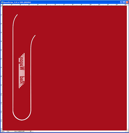
Figure 7-98: Flip the logo vertically, and save the image as its own file.
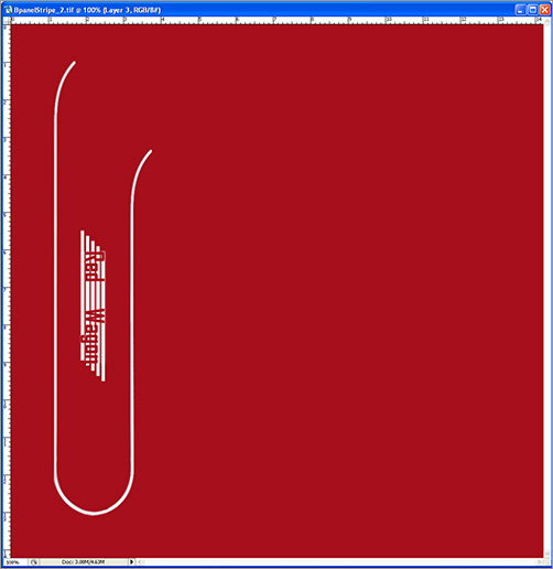
Figure 7-99: Assign the new image file to the new BpanelStripe1 shader.
4. Duplicate the BpanelStripe shader in the Hypershade by selecting the shader and choosing Edit ⇒ Duplicate ⇒ Shading Network. The copy is called BpanelStripe1.
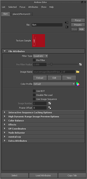
5. Select the newly copied BpanelStripe1 shader, and graph its input and output connections (![]() ) in the Hypershade. Select its file node, and open the Attribute Editor. Click the Folder icon to select a new image file, and then select the BpanelStripe_2.tif you just created in the Sourceimages folder. See Figure 7-99.
) in the Hypershade. Select its file node, and open the Attribute Editor. Click the Folder icon to select a new image file, and then select the BpanelStripe_2.tif you just created in the Sourceimages folder. See Figure 7-99.
6. The stripe and logo display on the wrong side of the B panel. Select the mesh, and center its pivot.
7. Set the Scale X attribute for the B panel to -1.0 to mirror it. The stripe and logo decals now show up on the correct side of the panel. Select the mesh, and freeze its transforms. Figure 7-100 shows the wagon so far.
Figure 7-100: The wagon has decals on both sides.

Texturing the Floor
Right now, the floor of the wagon is red, like the rest of its body. However, the real wagon has a blue floor, not red. If you select the mesh for the wagon’s floor (named wagonFloor) and assign the Blue shader you created, the whole body of the wagon turns blue, and that isn’t what you want. You only need the inside and bottom of the floor to be blue, not the front and back sides of the wagon’s body.
You’ll make a face assignment instead of dealing with UVs and image files. RMB+click the wagon floor mesh, and select Face from the marking menu. Select the two faces for the floor, as shown in Figure 7-101.
Figure 7-101: Select the floor faces.
With the faces selected, assign the Blue shader from the Hypershade window, and you’re done! You have a blue floor. All that remains now are the screws, bolts, handle, and wood railings.
You can load the file RedWagonTexture_v03.ma from the Scenes folder of the RedWagon project to check your work or skip to this point.
Shading the Wood Railings
You’ll go back to procedural shading and use the Wood texture available in Maya to create the wood railings, as you did with the axe exercise earlier in the chapter. Begin here:
1. In the Hypershade, create a new Phong material.
2. Click the Color Map icon (![]() ), and choose the Wood texture from the 3D Textures heading in the Create pane in the Hypershade.
), and choose the Wood texture from the 3D Textures heading in the Create pane in the Hypershade.
3. In the Attribute Editor for the Wood texture, set the Filler Color and Vein Color attributes according to Table 7-2.
Color and Vein Attributes
4. Set Vein Spread to 0.5, Layer Size to 0.5, Randomness to 1.0, Age to 10.0, and Grain Contrast to 0.33. In the Noise Attributes heading, set Amplitude X to 0.2 and Amplitude Y to 0.1, as shown in Figure 7-102. Name the shader wood.
5. Select all the wood railings and posts, and assign the Wood shader to them. Render a frame, and compare it to Figure 7-103. Notice the green cube place3dTexture node that is now in your scene. (See Figure 7-104.)
6. The side wood railings look fine; however, the wavy pattern on the front and back wood railings looks a bit odd. In the Hypershade, duplicate the shading network for the Wood shader, and call the new shader woodFront.
7. Assign that shader to the front and back railings and posts. Graph the network on the woodFront shader in the Hypershade window.
Figure 7-102: Setting the Wood texture

Figure 7-103: Assign the Wood shader.

Figure 7-104: The place3dTexture node for the wood texture

8. In the Hypershade, select the place3dTexture2 node (Figure 7-105) and the green cube in the view panels.
9. Rotate that placement node in the persp panel 90 degrees to the right or left. Render a frame, and compare it to Figure 7-106. The wood should no longer have that awkward wavy pattern.
Figure 7-105: Select the placement node for the second Wood texture.

Figure 7-106: The wood on the front and back railings looks better.
The wood railings are finished. Now, for some extra challenge, you can use pictures of real wood to map onto the railings for a more detailed look. The procedural Wood texture can give you only so much realism. If you create your own wood maps, use your experience with the side panels to create UV layouts for the railings so you can paint realistic wood textures using Photoshop. You’ll use custom photos and texture image maps next to simulate the rich wood in the decorative box.
Finishing the Wagon
Now that the railings are done and you have test renders, there are only two parts left to texture: the bullnose front of the wagon and the metal handle and screws. From here, take your time and create a bump map based on a fractal, as you did for the tires, and apply it to the bullnose’s black shader. Figure 7-107 shows a nice subtle bump map on the bullnose.
Figure 7-107: A nice bump for the bullnose
And last, you’ll need a metal shader for the screws, bolts, and handlebar for the wagon, just as you did for the axe exercise earlier in the chapter. Use a Phong shader with a blue-gray color and a low diffuse value, and assign it to all the metal parts of the wagon, as shown in Figure 7-108. You can then add an environment map to the reflection color, as you did for the axe earlier in this chapter to give the metal a reflective look.
Figure 7-108: Select all the metal screws, the bolts, and the handlebar, and assign the Metal shader to them.

Because metal is a tricky material to render, and a lot of metal’s look is derived from reflections, you’ll finish setting the Metal shader’s attributes in Chapter 11 when you render the wagon. You’ll enable raytracing to get realistic reflections and gauge how to best set up the Metal shader for a great look.
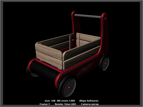
Figure 7-109 shows the wagon with all its parts assigned to shaders. Figure 7-110 shows a quick render of the wagon as it is now.
You can load the file RedWagonTexture_v04.ma from the Scenes folder of the RedWagon project to check your work or skip to this point.
Figure 7-109: The wagon in the Perspective panel
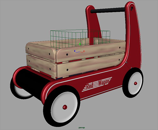
Figure 7-110: A current render of the wagon
