
SELECT A METHODOLOGY TO ESTIMATE THE MODEL
The selection of a certain methodology should pass the same quality tests as developing economic theories and selecting samples. Without strong intuition, researchers should choose the methodology that needs the least amount of human inputs. A good example is the machine-learning method that uses computerized algorithms to discover the knowledge (pattern or rule) inherent in data. Advances in modeling technology such as artificial intelligence, neural network, and genetic algorithms fit in this category. The beauty of this approach is its vast degree of freedom. There are none of the restrictions, which are often explicitly specified in traditional, linear, stationary models.
Of course, researchers should not rely excessively on the power of the method itself. Learning is impossible without knowledge. Even if you want to simply throw data into an algorithm and expect it to spit out the answer, you need to provide some background knowledge, such as the justification and types of input variables. There are still numerous occasions that require researchers to make justifiable decisions. For example, a typical way of modeling stock returns is using the following linear form,
- ERit = excess return for the ith security in period t
- Fjit−1 = jth factor value for the ith security at the beginning period t
- bkt = the market-wide payoff for factor k in period t
Trade-Off between Better Estimations and Prediction Errors
Undoubtedly, in testing and estimating equation (9.1), the first task is to decide which and how many explanatory variables should be included. This decision should not be a question whether the test is justified by a truly ex ante economic hypothesis. Economic theories, however, are often developed with abstract concepts that need to be measured by alternative proxies. The choice of proper proxies, while getting dangerously close to data snooping, makes the determination of both the type and the number of explanatory variables an art rather than a science. The choice of a particular proxy based on the rationale “Because it works!” is not sufficient unless it is first backed up by the theory.
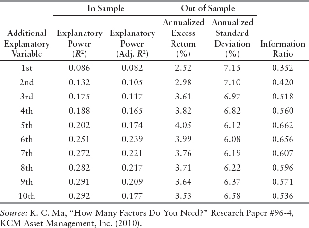
One rule of thumb is to be parsimonious. A big model is not necessarily better, especially in the context of predictable risk-adjusted excess return. While the total power of explanation increases with the number of variables (size) in the model, the marginal increase of explanatory power drops quickly after some threshold. Whenever a new variable is introduced, what comes with the benefit of the additional description is the increase of estimation error of an additional parameter. In Exhibit 9.2, we demonstrate the explanatory power of a typical multifactor model for stock returns by including one additional variable at a time from a study conducted by Ma in 2010.9 The second and the third columns clearly show that although by design the R-square increases with the number of the variables, the adjusted R-square, which also reflects the impact of the additional estimation error, levels off and starts decreasing after some point. This example suggests that in the process of estimation, the cost of estimation error is even compounded when new prediction is further extended into the forecast period. In Exhibit 9.2, we also perform out-of-sample prediction based on the estimated multifactor model in each stage. Columns 4 and 5 in the exhibit show a more striking pattern that the risk-adjusted excess return, in the form of information ratio, deteriorates even more quickly when the model becomes large.
EXHIBIT 9.2 Marginal Contribution of Additional Explanatory Variables
Animal Spirits
It is the exact same objectivity that quantitative analysts are proud of regarding their procedures that often leads to the question, “If everyone has the algorithms, will they not get the same answers?” The “overmining” on the same data set using simple linear models almost eliminates the possibility of gaining economic profit.
Pessimism resulting from the competition of quantitative research also justifies the need to include some form of “animal spirit” in the decision process. Being able to do so is also probably the single most important advantage that traditional security analysis can claim over quantitative approach. Casual observations provide ample examples that investor behavior determining market pricing follows neither symmetric nor linear patterns: investors tend to react to bad news much differently than to good news;10 information in more recent periods is overweighed in the decision process;11 investors ignore the probability of the event but emphasize the magnitude of the event;12 stocks are purchased for their glamour but not for intrinsic value;13 and, low PE stocks paying high returns do not imply that high price–earnings stocks pay low returns.14 We are not proposing that a quantitative model should include all these phenomenon, but the modeling methodology should be flexible enough to entertain such possibilities if they are warranted by the theory.
Statistical Significance Does Not Guarantee Economic Profits
As a result, staunch defenders of quantitative research argue that profitable strategies cannot be commercialized by quantitative analysis;15 the production of excess returns will stay idiosyncratic and proprietary. Profits will originate in those proprietary algorithms that outperform commercially standardized packages for data analysis. In other words, researchers will have to learn to gain confidence even if there is no statistical significance, while statistical significance does not guarantee economic profit.
Since quantitative market strategists often start with the identification of a pattern that is defined by statistical standards, it is easy to assume economic profit from conventional statistical significance. To show that there is not necessarily a link, we perform a typical momentum trading strategy that is solely based on the predictability of future returns from past returns. A simplified version of the return-generating process under this framework follows:
![]()
where Et-1(Rt) is the expected return for the period t, estimated at point t – 1, a is time-invariant return, and bt-1 is the momentum coefficient observed at time t-1. When bt-1 is (statistically) significantly positive, the time-series returns are said to exhibit persistence and positive momentum. To implement the trading strategy using the information in correlations, stocks with at least a certain level of correlation are included in portfolios at the beginning of each month, and their returns are tracked. The performance of these portfolios apparently reflects the statistical significance (or lack of) in correlation between successive returns. In Exhibit 9.3, we summarize the performance of some of the representative portfolios from a study conducted and updated by Ma in 2005 and 2010.16
EXHIBIT 9.3 Statistical Significance and Economic Profits
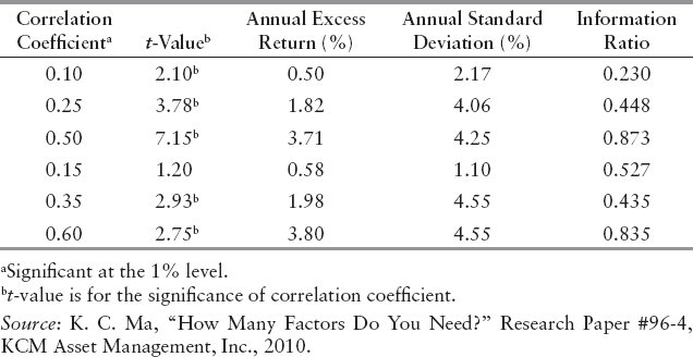
It is not surprising that higher excess returns are generally associated with higher correlation between successive returns. More importantly, higher risk seems to be also related to higher statistical significance of the relationship (correlation). The bottom line is that an acceptable level of risk-adjusted excess return, in the form of information ratio (e.g., 1), cannot always be achieved by statistical significance alone. A more striking observation, however, is that, sometime without conventional statistical significance, the portfolio was able to deliver superior risk-adjusted economic profit. While the driving force may yet be known, evidence is provided for the disconnection between statistical significance and economic profit.
A Model to Estimate Expected Returns
The estimation for the model to explain past returns from Step 3, by itself, is not enough, since the objective of the process is to predict future returns. A good model for expected return is much harder to come by since we simply don't have enough data. As pointed out by Fischer Black, people are often confused between a model to explain average returns and a model to predict expected returns.17 While the former can be tested on a large number of historical data points, the latter requires such a long time period (sometimes decades) to cover various conditions to predict the expected return. Since we do not have that time to wait, one common shortcut is to simply assume that the model to explain average returns will be the model to predict expected returns. Of course, such prediction is highly inaccurate, given the assumption of constant expected returns.
We can easily find evidence to show it is a bad assumption. For example, if one can look at the actual model that explains the cross-sections of short-term stock returns, even the most naive researcher can easily conclude that there is little resemblance between the models from one period to the next. This would in turn suggest, at least in the short term, the model to explain past returns cannot be used to predict expected returns.
We are calling for brand new efforts to establish an ex ante expected return model. The process has to pass the same strict tests for quality that are required for any good modeling, as discussed earlier. These tests would include the independent formulation of the hypothesis for expected return and a methodology and sample period free from data snooping and survivorship bias. While they are not necessarily related, the process of developing hypotheses for conditional expected return models can greatly benefit from the insights from numerous models of past returns estimated over a long time period.
Largest Value Added
Apparently, the final risk-adjusted returns from a strategy can be attributed to the proper execution of each step described in Exhibit 9.1. The entire process can be generally described in a three-step procedure consisting of economic hypothesis, model estimation, and prediction. It is only natural for researchers to ask how to allocate their efforts among the three steps to maximize the return contribution.
To answer this question, we examine the return contribution from model estimation and prediction. For this purpose, we use a typical multifactor model to explain the return for all stocks in the Standard & Poor's 500 Index. Assume that at the beginning of each period, the best model actually describing the return in the period is known to the portfolio manager. Using this information, a portfolio consisting of the predicted top quartile is formed. The excess return from this portfolio generated with perfect information would suggest the extent of return contribution from model estimation. Accordingly, based on a 2010 study by Ma18 reported in Exhibit 9.4, the annual mean excess return of the top predicted quartile is between 12% and 26%, depending on the length of the investment horizon.
EXHIBIT 9.4 Potential Returns for Perfect Estimation and Prediction: S&P 500 Stocks, 1975—2010

In contrast, the annual mean excess return of the actual top quartile in the S&P 500 Index is between 42% and 121%. The difference in excess return between the actual top quartile portfolio and the predicted top quartile portfolio, between 30% and 95%, would suggest the extent of the return contribution from model prediction. It is clear then that for all investment horizons, the return contribution from model prediction is on average two to five times the excess returns from model estimation.
Therefore, for all practical purposes, the step of identifying a predictable model is responsible for the largest potential value added in generating predictable excess returns. The implication is that resources allocated to research should be placed disproportionally toward the effort of out-of-sample prediction.
Test the Prediction Again!
Another safeguard against data snooping is to scrutinize the model once more through time. That is, the conditional model to estimate expected return needs to be tested again in a “fresh” data period. As it requires multiple time periods to observe the conditional model for expected returns, the prediction model derived under a single condition has to be confirmed again. In Exhibit 9.5, we specify the relationship in time periods among estimation, testing, and confirmation.

The sequential testing of the prediction model in the forecast period would affirm the condition that converts the model of actual returns to the model of expected returns still produces an acceptable level of performance. As the conditioning factor varies from one period to anther, the consistent performance of the three-period process suggests that it is not driven by a constant set of artificial rules introduced by data snooping.
Test against a Random Walk
After completing the modeling exercise it is always wise to test the model against an artificial data set formed from independent and identically distributed returns. Any trading strategy applied to purely random data should yield no average profit. Of course, purely random fluctuations will produce profits and losses. However, because we can simulate very long sequences of data, we can test with high accuracy that our models do not actually introduce artefacts that will not live up to a real life test.