HYPOTHETICAL EXAMPLE

Suppose that an analyst is seeking to gauge whether Company A is attractive or unattractive, on the basis of relative valuation methods. Suppose that the analyst has determined that there are six other listed companies in the same industry that are approximately the same size and comparable in terms of product mix, client base, and geographical focus.²⁰ Based on this information, the analyst can calculate some potentially useful multiples for all seven companies. A hypothetical table of such results is shown in Exhibit 4.1. (For the purposes of this simple hypothetical example, we are assuming that all the firms have the same fiscal year. We consider calendarization later in this chapter.)

EXHIBIT 4.1 Hypothetical Relative Valuation Results

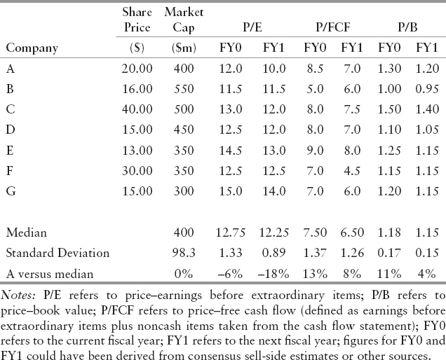
In this hypothetical scenario, Company A is being compared to companies B through G, and, therefore, Company A should be excluded from the calculation of median and standard deviation, to avoid double-counting. The median is used because it tends to be less influenced by outliers than the statistical mean, so it is likely to be a better estimate for the central tendency. (Similarly, the standard deviation can be strongly influenced by outliers, and it would be possible to use “median absolute deviation” as a more robust way of gauging the spread around the central tendency. Such approaches may be particularly appropriate when the data contains one or a handful of extreme outliers for certain metrics, which might be associated with company-specific idiosyncrasies.) Exhibit 4.1 has been arranged in terms of market cap, from largest to smallest, which can sometimes reveal patterns associated with larger or smaller firms, though there don't appear to be any particularly obvious trends in this particular set of hypothetical numbers.

Exhibit 4.1 suggests that the chosen universe of comparable companies may be reasonably similar to Company A in several important respects. In terms of size, Companies B, C, and D are slightly larger, while Companies E, F, and G are slightly smaller, but the median market cap across the six firms is the same as Company A's current valuation. In terms of P/E ratios, Company A looks slightly cheap in terms of FY0 earnings and somewhat cheaper in terms of FY1 earnings. In terms of P/FCF ratios, Company A looks somewhat expensive in terms of FY0 free cash flow, but only slightly expensive in terms of FY1 free cash flow. And finally, in terms of P/B ratios, Company A looks somewhat expensive in terms of FY0 book value, but roughly in line with its peers in terms of FY1 book value.

Analysis of the Hypothetical Example

So what are the implications of these results? Firstly, Company A looks relatively cheap compared to its peer group in terms of P/E ratios, particularly in terms of its FY1 multiples. Secondly, Company A looks rather expensive compared to its peer group in terms of P/FCF and P/B ratios, particularly in terms of FY0 figures. If an analyst were focusing solely on P/E, then Company A would look cheap compared with the peer group, and this might suggest that Company A could be an attractive investment opportunity.

However, the analyst might be concerned that Company A looks comparatively cheap in terms of P/E, but somewhat expensive in terms of price–book value. One way to investigate this apparent anomaly is to focus on ROE, which is defined as earnings–book value. Using the data in Exhibit 4.1, it is possible to calculate the ROE for Company A and for the other six companies, by dividing the P/B ratio by the P/E ratio—because this effectively cancels out the “price” components, and thus will generate an estimated value for EPS divided by book value per share, which is one way to calculate ROE.

The results suggest that Company A is expected to deliver an ROE of 10.8% in FY0 and 12% in FY1, whereas the median ROE of the other six firms is 8.7% in FY0 and 8.8% in FY1. Most of the comparable companies are expected to achieve ROE of between 8% and 9% in both FY0 and FY1, though apparently Company C is expected to achieve ROE of 11.5% in FY0 and 11.7% in FY1. (A similar analysis can be conducted using “free cash flow to equity,” which involves dividing the P/B ratio by the P/FCF ratio. This indicates that Company A is slightly below the median of Companies B through G in FY0, but in line with its six peers during FY1.)

These results suggest that Company A is expected to deliver an ROE that is substantially higher than most of its peers. Suppose that an analyst is skeptical that Company A really can deliver such a strong performance, and instead hypothesizes that Company A's ROE during FY0 and FY1 may only be in line with the median ROE for the peer group in each year. Based on the figures in Exhibit 4.1, Company A's book value in FY0 is expected to be $15.38, and the company is projected to deliver $1.67 of earnings. Now suppose that Company A's book value remains the same, but that its ROE during FY0 is only 8.7%, which is equal to the median for its peers. Then the implied earnings during FY0 would only be $1.35, and the “true” P/E for Company A in FY0 would be 14.9, well above the peer median of 12.75.

The analysis can be extended a little further, from FY0 to FY1. The figures in Exhibit 4.1 suggest that Company A's book value in FY1 will be $16.67, and that the company will generate $2.00 of earnings during FY1. But if Company A only produced $1.35 of earnings during FY0, rather than the table's expectation of $1.67, then the projected FY1 book value may be too high. A quick way to estimate Company A's book value in FY1 is to use a “clean surplus” analysis, using the following equation:

Based on the figures in Exhibit 4.1, Company A is expected to have earnings of $1.67 during FY0, and $2.00 during FY1. The implied book value per share is $15.38 in FY0, and $16.67 during FY1. According to the clean surplus formula, Company A is expected to pay a dividend of $0.38 per share in FY1.

Assuming that the true earnings in FY0 are indeed $1.35 rather than $1.67, and that the dividend payable in FY1 is still $0.38, then the expected book value for Company A in FY1 would be $16.35 rather than $16.67. Taking this figure and applying the median FY1 peer ROE, the expected FY1 earnings for Company A would be $1.42 rather than $2.00, and consequently the “true” P/E for FY1 would be 13.9 instead of the figure of 10.0 shown in Exhibit 4.1. At those levels, the stock would presumably no longer appear cheap by comparison with its peer group. Indeed, Company A's FY1 P/E multiple would be roughly in line with Company G, which has the highest FY1 P/E multiple among the comparable companies.

This quick analysis therefore suggests that the analyst may want to focus on why Company A is expected to deliver FY0 and FY1 ROE, which is at or close to the top of its peer group. As noted previously, Company A and Company C are apparently expected to have ROE, which is substantially stronger than the other comparable companies. Is there something special about Companies A and C that would justify such an expectation? Conversely, is it possible that the estimates for Companies A and C are reasonable, but that the projected ROE for the other companies is too pessimistic? If the latter scenario is valid, then it's possible that the P/E ratios for some of the other companies in the comparable universe are too high, and thus that those firms could be attractively valued at current levels.

Other Potential Issues

Multiples Involving Low or Negative Numbers

It is conventional to calculate valuation multiples with the market valuation as the numerator, and the firms' financial or operating data as the denominator. If the denominator is close to zero, or negative, then the valuation multiple may be very large or negative. The simplest example of such problems might involve a company's earnings. Consider a company with a share price of $10 and projected earnings of $0.10 for next year. Such a company is effectively trading at a P/E of 100. If consensus estimates turn more bearish, and the company's earnings next year are expected to be minus $0.05, the company will now be trading at a P/E of −200.

It is also possible for a firm to have negative shareholders' equity, which would indicate that the total value of its liabilities exceeds the value of its assets. According to a normal understanding of accounting data, this would indicate that the company is insolvent. However, some companies have been able to continue operating under such circumstances, and even to retain a stock exchange listing. Firms with negative shareholders' equity will also have a negative price–book multiple. (In principle, a firm can even report negative net revenues during a particular period, though this would require some rather unusual circumstances. One would normally expect few firms to report negative revenues for more than a single quarter.)

As noted previously, averages and standard deviations tend to be rather sensitive to outliers, which is one reason to favor using the median and the median absolute deviation instead. But during economic recessions at the national or global level, many companies may have low or negative earnings. Similarly, firms in cyclical industries will often go through periods when sales or profits are unusually low, by comparison with their average levels through a complete business cycle. Under such circumstances, an analyst may prefer not to focus on conventional metrics such as price–earnings, but instead to use line items from higher up the income statement that will typically be less likely to generate negative numbers.

Calendarization

Some of the firms involved in the relative valuation analysis may have fiscal years that end on different months. Most analyst estimates are based on a firm's own reporting cycle. It is usually desirable to ensure that all valuation multiples are being calculated on a consistent basis, so that calendar-based effects are not driving the analysis.

One way to ensure that all valuation multiples are directly comparable is to calendarize the figures. Consider a situation where at the start of January, an analyst is creating a valuation analysis for one firm whose fiscal year ends in June, while the other firms in the universe have fiscal years that end in December. Calendarizing the results for the June-end firm will require taking half of the projected number for FY0, and adding half of the projected number for FY1. (If quarter-by-quarter estimates are available, then more precise adjustments can be implemented by combining 3QFY0, 4QFY0, 1QFY1, and 2QFY1.)

Calendarization is conceptually simple, but may require some care in implementation during the course of a year. One would expect that after a company has reported results for a full fiscal year, the year defined as “FY0” would immediately shift forward 12 months. However, analysts and data aggregators may not change the definitions of “FY0” and “FY1” for a few days or weeks. In case of doubt, it may be worth looking at individual estimates in order to double-check that the correct set of numbers is being used.

Sum-of-the-Parts Analysis

When attempting to use relative valuation methods on firms with multiple lines of business, the analyst may not be able to identify any company that is directly similar on all dimensions. In such instances, relative valuation methods can be extended to encompass “sum-of-the-parts” analysis, which considers each part of a business separately, and attempts to value them individually by reference to companies that are mainly or solely in one particular line of business.²¹

Relative valuation analysis based on sum-of-the-parts approaches will involve the same challenges as were described above—identifying a suitable universe of companies that are engaged in each particular industry, collecting and collating the necessary data, and then using the results to gauge what might be a “fair value” for each of the individual lines of business. But in addition to these considerations, there is an additional difficulty that is specific to sum-of-the-parts analysis. This problem is whether to apply a “conglomerate discount,” and if so how much.

Much financial theory assumes that all else equal, investors are likely to prefer to invest in companies that are engaged in a single line of business, rather than to invest in conglomerates that have operations across multiple industries. Investing in a conglomerate effectively means being exposed to all of that conglomerate's operations, and the overall mix of industry exposures might not mimic the portfolio that the investor would have chosen if it were possible instead to put money into individual companies.

A possible counterargument might be that a conglomerate with strong and decisive central control may achieve synergies with regard to revenues, costs or taxation would not be available to individual free-standing firms dealing at arms' length with each other. A skeptical investor might wonder, on the other hand, about whether the potential positive impact of such synergies may be partly or wholly undermined by the negative impacts of centralized decision making, transfer pricing, and regulatory or reputational risk.

For these reasons, an analyst might consider that it is reasonable to apply a discount to the overall value that emerges from the “sum of the parts.” Some practitioners favor a discount of somewhere between 5% and 15%, for the reasons given earlier. Academic research on spinoffs has suggested that the combined value of the surviving entity and the spun-off firm tends to rise by an average of around 6%, though with a wide range of variation.²² (Some analysts have suggested that in some particular contexts, for instance in markets where competent managers are very scarce, then investors should be willing to pay a premium for being able to invest in a conglomerate that is fortunate enough to have such executives. However, this appears not to be a mainstream view.)

Relative Valuation vs. DCF: A Comparison

Relative valuation methods can generally be implemented fairly fast, and the underlying information necessary to calculate can also be updated quickly. Even with the various complexities discussed above, an experienced analyst can usually create a relative valuation table within an hour or two. And the calculated valuation multiples can adjust as market conditions and relative prices change. In both respects, relative valuation methods have an advantage over DCF models, which may require hours or days of work to build or update, and that require the analyst to provide multiple judgment-based inputs about unknowable future events. Moreover, as noted by Baker and Ruback, if a DCF model is extended to encompass multiple possible scenarios, it may end up generating a range of “fair value” prices that is too wide to provide much insight into whether the potential investment is attractive at its current valuation.²³

Relative valuation methods focus on how much a company is worth to a minority shareholder, in other words an investor who will have limited or zero ability to influence the company's management or its strategy. Such an approach is suitable for investors who intend to purchase only a small percentage of the company's shares, and to hold those shares until the valuation multiple moves from being “cheap” to being “in line” or “expensive” compared with the peer group. As noted above, relative valuation methods make no attempt to determine what is the “correct” price for a company's shares, but instead focuses on trying to determine whether a company looks attractive or unattractive by comparison with other firms that appear to be approximately similar in terms of size, geography, industry, and other parameters.

DCF methods attempt to determine how much a company is worth in terms of “fair value” over a long time horizon. DCF methods can readily incorporate a range of assumptions about decisions in the near future or the distant future, and therefore can provide a range of different scenarios. For this reason, most academics and practitioners consider that DCF methods are likely to produce greater insight than relative valuation methods into the various forces that may affect the fair value for a business. More specifically, DCF methods can be more applicable to situations where an investor will seek to influence a company's future direction—perhaps as an activist investor pushing management in new directions, or possibly as a bidder for a controlling stake in the firm. In such situations, relative valuation analysis is unlikely to provide much insight because the investor will actually be seeking to affect the company's valuation multiples directly, by affecting the value of the denominator.

Nevertheless, even where an analyst favors the use of DCF approaches, we consider that relative valuation methods can still be valuable as a “sanity check” on the output from a DCF-based valuation. An analyst can take the expected valuation from the DCF model, and compare it with the projected values for net income, shareholders' equity, operating cash flow, and similar metrics. These ratios drawn from the DCF modeling process can then be compared with the multiples for a universe of similar firms. If the multiples that are generated by the analyst's DCF model are approximately comparable with the multiples that can be derived for similar companies already being publicly traded, then the analyst may conclude that the DCF model's assumptions appear to be reasonable. However, if the multiples from the analyst's model appear to diverge considerably from the available information concerning valuation multiples for apparently similar firms, then it may be a good idea to reexamine the model, rechecking whether the underlying assumptions are truly justifiable.

Relative valuation methods can also be useful in another way when constructing DCF models. Most DCF models include a “terminal value” that represents the expected future value of the business, discounted back to the present, from all periods subsequent to the ones for which the analyst has developed explicit estimates. One way to calculate this terminal value is in terms of a perpetual growth rate, but the choice of a particular growth rate can be difficult to justify on the basis of the firm's current characteristics. An alternative approach is to take current valuation multiples for similar firms, and use those values as multiples for terminal value.²⁴