INCORPORATING TRANSACTION COSTS

Transaction costs can be generally divided into two categories: explicit (such as bid-ask spreads, commissions and fees), and implicit (such as price movement risk costs⁹ and market impact costs¹⁰).

The typical portfolio allocation models are built on top of one or several forecasting models for expected returns and risk. Small changes in these forecasts can result in reallocations that would not occur if transaction costs are taken into account. In practice, the effect of transaction costs on portfolio performance is far from insignificant. If transaction costs are not taken into consideration in allocation and rebalancing decisions, they can lead to poor portfolio performance.

This section describes some common transaction cost models for portfolio rebalancing. We use the mean-variance framework as the basis for describing the different approaches. However, it is straightforward to extend the transaction cost models into other portfolio allocation frameworks.

The earliest, and most widely used, model for transaction costs is the mean-variance risk-aversion formulation with transaction costs.¹¹ The optimization problem has the following objective function:

where TC is a transaction cost penalty function, and λ_TC is the transaction cost aversion parameter. In other words, the objective is to maximize the expected portfolio return less the cost of risk and transaction costs. We can imagine that, as the transaction costs increase, at some point it becomes optimal to keep the current portfolio rather than to rebalance. Variations of this formulation exist. For example, it is common to maximize expected portfolio return minus transaction costs and impose limits on the risk as a constraint (i.e., to move the second term in the objective function in the constraints).

Transaction costs models can involve complicated nonlinear functions. Although software exists for general nonlinear optimization problems, the computational time required for solving such problems is often too long for realistic investment applications, and the quality of the solution is not guaranteed. In practice, an observed complicated nonlinear transaction costs function is often approximated with a computationally tractable function that is assumed to be separable in the portfolio weights, that is, it is often assumed that the transaction costs for each individual stock are independent of the transaction costs for another stock. For the rest of this section, we denote the individual cost function for stock i by TC_i.

Next, we explain several widely used models for the transaction cost function.

Linear Transaction Costs

Let us start simple. Suppose that the transaction costs are proportional, that is, they are a percentage c_i of the transaction size |t| = |w_i − w_0,i|.¹² Then, the portfolio allocation problem with transaction costs can be written simply as

The problem can be made solver-friendly by replacing the absolute value terms with new decision variables y_i, and adding two sets of constraints. Hence, we rewrite the objective function as

and add the constraints

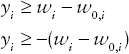
This preserves the quadratic optimization problem formulation, a formulation that can be passed to quadratic optimization solvers such as Excel Solver and MATLAB's quadprog function, because the constraints are linear expressions, and the objective function contains only linear and quadratic terms.

In the optimal solution, the optimization solver will in fact set the value for y_i to |w_i − w_0,i|. This is because this is a maximization problem and y_i occurs with a negative sign in the objective function, so the solver will try to set y_i to the minimum value possible. That minimum value will be the maximum of (w_i – w_0,i) or −( w_i – w_0,i), which is in fact the absolute value |w_i − w_0,i|.

Piecewise-Linear Transaction Costs

Taking the model in the previous section a step further, we can introduce piecewise-linear approximations to transaction cost function models. This kind of function is more realistic than the linear cost function, especially for large trades. As the trading size increases, it becomes increasingly more costly to trade because of the market impact of the trade.

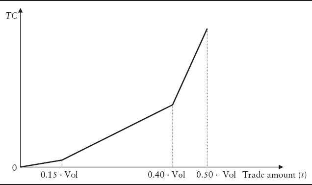
An example of a piecewise-linear function of transaction costs for a trade of size t of a particular security is illustrated in Exhibit 18.1. The transaction cost function in the graph assumes that the rate of increase of transaction costs (reflected in the slope of the function) changes at certain threshold points. For example, it is smaller in the range 0% to 15% of daily volume than in the range 15% to 40% of daily volume (or some other trading volume index). Mathematically, the transaction cost function in Exhibit 18.1 can be expressed as

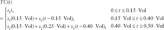
where s₁, s₂, s₃ are the slopes of the three linear segments on the graph. (They are given data.)

EXHIBIT 18.1 Example of Modeling Transaction Costs (TC) as a Piecewise-Linear Function of Trade Size t

To include piecewise-linear functions for transaction costs in the objective function of a mean-variance (or any general mean-risk) portfolio optimization problem, we need to introduce new decision variables that correspond to the number of pieces in the piecewise-linear approximation of the transaction cost function (in this case, there are three linear segments, so we introduce variables z₁, z₂, z₃). We write the penalty term in the objective function for an individual stock as:¹³

If there are N stocks in the portfolio, the total transaction cost will be the sum of the transaction costs for each individual stock, that is, the penalty term that involves transaction costs in the objective function becomes

In addition, we specify the following constraints on the new decision variables:

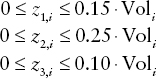
Note that because of the increasing slopes of the linear segments and the goal of making that term as small as possible in the objective function, the optimizer will never set the decision variable corresponding to the second segment, z_2,i, to a number greater than 0 unless the decision variable corresponding to the first segment, z_1,i, is at its upper bound. Similarly, the optimizer would never set z_3,i to a number greater than 0 unless both z_1,i and z_2,i are at their upper bounds. So, this set of constraints allows us to compute the amount of transaction costs incurred in the trading of stock i as z_1,i + z_2,i + z_3,i.

Of course, we also need to link the amount of transaction costs incurred in the trading of stock i to the optimal portfolio allocation. This can be done by adding a few more variables and constraints. We introduce variables y_i, one for each stock in the portfolio, that would represent the amount traded (but not the direction of the trade), and would be nonnegative. Then, we require that

and also that y_i equals the change in the portfolio position of stock i. The latter condition can be imposed by writing the constraint

where w_0,i and w_i are the initial and the final amount of stock i in the portfolio, respectively.¹⁴

Despite their apparent complexity, piecewise-linear approximations for transaction costs are very solver-friendly, and save time (relative to nonlinear models) in the actual portfolio optimization. Although modeling transaction costs this way requires introducing new decision variables and constraints, the increase in the dimension of the portfolio optimization problem does not affect significantly the running time or the performance of the optimization solver, because the problem formulation is easy from a computational perspective.

Quadratic Transaction Costs

The transaction cost function is often parameterized as a quadratic function of the form

The coefficients c_i and d_i are calibrated from data, such as fitting a quadratic function to an observed pattern of transaction costs realized for trading a particular stock under normal conditions.

Including this function in the objective function of the portfolio optimization problem results in a quadratic program that can be solved with widely available quadratic optimization software.

Fixed Transaction Costs

In some cases, we need to model fixed transaction costs. Those are costs that are incurred independently of the amount traded. To include such costs in the portfolio optimization problem, we need to introduce binary variables δ₁, …, δ_N corresponding to each stock, where δ_i equals 0 if the amount traded of stock i is 0, and 1 otherwise. The idea is similar to the idea we used to model the requirement that only a given number of stocks can be included in the portfolio.

Suppose the fixed transaction cost is a_i for stock i. Then, the transaction cost function is

The objective function formulation is then

and we need to add the following constraints to make sure that the binary variables are linked to the trades |w_i − w_0,i|:

where M is a “large” constant. When the trading size |w_i − w_0,i| is nonzero, δ_i will be forced to be 1. When the trading size is 0, then δ_i can be either 0 or 1, but the optimizer will set it to 0, since it will try to make its value the minimum possible in the objective function.

Of course, combinations of different trading cost models can be used in practice. For example, if the trade involves both a fixed and a variable quadratic transaction cost, then we could use a transaction cost function of the kind

The important takeaway from this section is that when transaction costs are included in the portfolio rebalancing problem, the result is a reduced amount of trading and rebalancing, and a different portfolio allocation than the one that would be obtained if transaction costs are not taken into consideration.