OVERVIEW OF VALUE-BASED METRICS

We now provide an overview of VBM. Value-based metrics are financial measures that largely evolve out of corporate finance. The focus here is on metrics that can assist managers and investors in discerning whether a company is pointing in the direction of wealth creation or, unfortunately, wealth destruction. In the VBM approach to fundamental analysis, the focus is on discovering firms that can consistently earn a return on capital (ROC) that exceeds the weighted average cost of capital (WACC).

A financial metric takes on a VBM character when there is an explicit recognition of and accounting for the overall cost of capital (WACC in the economic value added model described below) or the cost of equity (r in the residual income or abnormal earnings model also described below). Hence, the most distinctive feature of VBM analysis (in contrast to traditional analysis) is the formal recognition of the investor's required rate of return (cost of equity) and the overall cost of capital. Value-based metrics include:

• Residual income (abnormal earnings)
• Residual income spread
• Economic value added (EVA^®)
• Economic value added spread
• Market value added (MVA)
• Cash flow return on investment (CFROI^®)

Background

We'll begin the VBM approach to equity analysis with a metric called economic value added (EVA). EVA was developed commercially in the early 1980s by Joel Stern and G. Bennett Stewart III. This economic profit measure gained early acceptance in the corporate community because of its innovative way of looking at profit net of the overall dollar cost of capital, including debt and equity capital costs. EVA principles have been used by many companies to design incentive compensation programs that provide value-based incentives for managers (agents) to make wealth-enhancing decisions for the shareholders (principals).

In turn, EVA gained popularity in the investment community with the establishment in 1996 of CS First Boston's annual conference on economic value added. In 1997, the U.S. Equity Research Group at Goldman Sachs developed an EVA platform to evaluate the performance of companies, industries, and sectors of the economy. On the buy side, Centre Asset Management LLC and EVA Advisors LLC are two examples of today's investment firms that use an EVA approach to select stocks and build long-short equity portfolios.

The financial significance of using EVA to evaluate company and stock performance is crystal clear: Wealth-creating firms have positive EVA because their NOPAT exceeds the dollar weighted average cost of capital. Wealth destroyers lose market value and incur share price decline because their corporate profitability falls short of the capital costs. This wealth loss can occur even though the firm's accounting profit is positive. This happens when pretax operating earnings (EBIT) are sufficient enough to cover debt-interest costs, but they are not high enough to cover the combined dollar costs of debt and equity financings. Herein lay a key distinction between accounting-based traditional metrics and value-based metrics.

Basic EVA

Central to the EVA calculation is the concept of levered and unlevered firms. A “levered” firm, like most real-world firms, is one that partly finances its growth opportunities with long-term debt. In contrast, an equivalent-risk “unlevered” firm is financed by 100% equity. This firm-type classification is helpful because EVA is calculated by subtracting the firm's dollar weighted average cost of debt and equity capital ($WACC) from its unlevered NOPAT.

NOPAT is used in the EVA formulation for two reasons. First, emphasis on this term serves as a reminder that the firm largely receives its profitability from the desirability of its products and services. Second, since most firms have some form of debt outstanding, they receive a yearly interest tax subsidy—measured by the corporate tax rate times the interest expense—that is already reflected in the dollar cost of capital.

This second point is important. An incorrect focus by managers or investors on the levered firm's net operating profit after taxes, LNOPAT, rather than its unlevered profit measure, NOPAT, would lead to an upward bias in the firm's economic value added. By avoiding the double counting of the firm's yearly interest tax subsidy, the investor avoids imparting a positive bias in not only the firm's profitability but also its enterprise value and underlying stock price.

In basic terms, NOPAT can be expressed as (1) tax-adjusted operating earnings (EBIT) or (2) net income (NI) plus after-tax interest expense according to

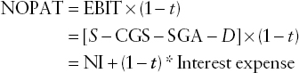
In the first expression, NOPAT is shown as tax-adjusted operating earnings, EBIT × (1 − t). EBIT in the second expression is sales less cost of goods sold, selling, general, and administrative expenses, and depreciation. In principle, depreciation should be a charge that reflects the economic obsolescence of the firm's operating assets. In the third expression, the analyst or investor begins with accounting net income and adds back the after-tax interest expense to work back to tax-adjusted operating earnings, EBIT × (1 − t).

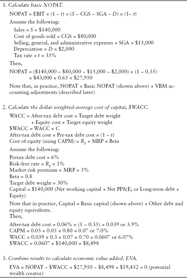
In turn, the firm's $WACC can be expressed as

In this expression, %WACC is the firm's percentage weighted average cost of debt and equity capital, while the letter C is its operating capital. Note that capital can be expressed in terms of operating assets (such as net short-term operating assets plus net plant, property, and equipment) or financing capital (reflecting debt and equity financings). The cost of capital percentage is given by

With NOPAT expressed as tax-adjusted operating earnings, we see that a firm's basic EVA can be expressed as

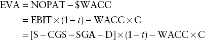
This expression shows that the firm's EVA is equal to its NOPAT less the dollar cost of all capital employed in the business. Moreover, the EVA formula suggests at least five ways to increase a company's economic earnings. These include:

1. Increase revenue (growth).
2. Reduce operating expenses where prudent.
3. Use less capital to produce the same amount of goods and services (improved capital turnover ratios).
4. Use more capital in the presence of positive EVA growth opportunities.
5. Reduce WACC (via greater consistency of earnings and cash flows).

Exhibit 2.5 provides a three-part example on how to estimate basic EVA. The table shows how to estimate the three components of EVA, including NOPAT, WACC, and capital. In this illustration, the firm is pointing in the direction of value creation because its economic profit is positive. Likewise, in EVA spread terms, the firm is a potential wealth creator because its after-tax ROC is higher than its cost of capital.

In practice, there are numerous accounting adjustments that investors should be aware of when estimating EVA via NOPAT and capital. We cover some of the more popular ones at the end of our VBM survey. In the next few sections, we'll discuss related VBM metrics and concepts including (1) how to measure the EVA spread, (2) how to decompose ROC into profit margins and capital turns, (3) WACC issues, (4) cash flow return on investment, (5) residual income (abnormal earnings), and (6) the role of EVA and residual income momentum in discerning “good companies” from “bad” or risky-troubled companies and related stock valuation considerations. Finally, the appendix provides a case study on how to combine traditional and value-based metrics to come up with an integrated, overall stock rating.

EVA Spread

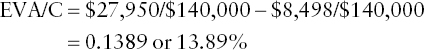
VBM can be expressed in either dollar or ratio terms. One of the more popular ratio (or percentage) forms is the EVA spread. This is also referred to as the residual ROC (or surplus rate of return on capital). The EVA spread is simply the return on capital less WACC. The EVA spread is obtained by dividing EVA by capital to obtain:

EXHIBIT 2.5 Three-Part Calculation of EVA

With this expression, an investor can assess whether a company is pointing in the direction of wealth creation, wealth neutrality, or wealth destruction. If the EVA spread is positive, the firm is a potential value creator, since ROC exceeds WACC. Conversely, if ROC is less than WACC, the firm points in the direction of value destruction, even though reported accounting earnings may be positive. While such a firm may meet its debt interest expense, it is unable to account for the opportunity cost of equity, whether measured in dollar or ratio terms. The EVA spread in the example given in Exhibit 2.5 is 13.89% as shown:

The EVA spread is positive and attractive because the ROC, at 19.96%, is considerably higher than the WACC, at 6.07%.

Return on Capital Decomposition

Like ROA in the Dupont model, ROC can be expressed in terms of an operating profit margin and a capital turnover ratio:

Moreover, since C (assets perspective) is equal to net short-term operating assets (NWC less short-term debt) plus net plant, property, and equipment, we can express ROC in terms of an operating margin and working capital and NPPE turns:

Not surprisingly, higher operating margins, higher net working capital, and net plant and equipment (including technology) turns lead to higher ROC. Assuming that WACC remains unchanged, the higher ROC leads to a higher EVA spread. This leads to higher EVA and, if sustainable, higher enterprise value—especially with capital expansion (role discussed shortly), assuming that this information is not already reflected in share price.

From Exhibit 2.5, the NOPAT margin (NOPAT/S) is coincidentally the same as ROC, at 19.96%. This happens because the capital turnover ratio (S/C) is unity:

WACC Issues

Central to the VBM model is the recognition that a firm is not truly profitable unless it earns a return on capital that exceeds the opportunity cost of capital. That being said, questions remain about the actual calculation of WACC. We provide an overview of two particular controversies that present real-world challenges to estimating WACC. These issues pertain to (1) the debt weight (and therefore equity weight) used in the EVA formulation and (2) how to estimate the investor's required rate of return (cost of equity).

Target Capital Structure

One of the major issues in the real-world application of EVA (or residual income) analysis is the question of capital structure. For our purposes, capital structure refers to the debt and equity weights that an investor or analyst should use in the EVA formulation. The question of a target capital structure—reflecting a presumed “optimal” mix of debt and equity financings—is a long-standing debate in the theory of corporate finance. Exhibit 2.6 provides a graphical depiction of the capital structure issue in terms of the traditional view of capital structure versus the Modigliani-Miller view (a celebrated theory proposed in 1958 with subsequent variation). The original theory by Modigliani and Miller (MM) can be interpreted as a special case of the VBM approach to capital structure.

EXHIBIT 2.6 Impact of Capital Structure Change on Enterprise Value

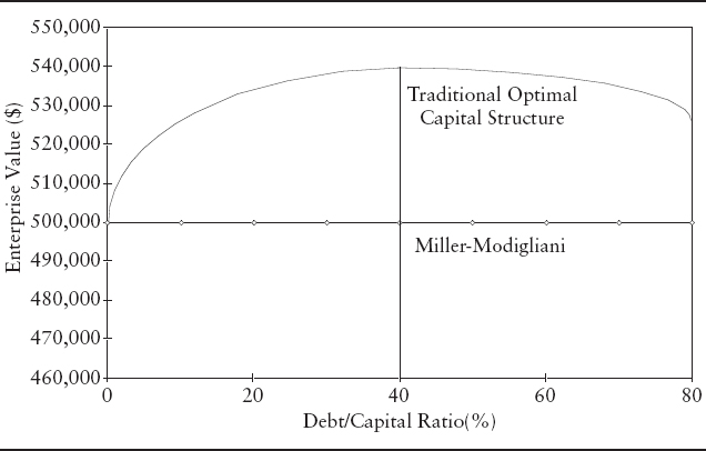
Exhibit 2.6 shows the pricing implications of the traditional versus MM views of capital structure, measured in terms of corporate value (vertical axis) and leverage (horizontal axis). In general, V_u is the market value of the unlevered firm—a firm having no long-term debt—while V_l denotes the market value of a levered firm—a firm with debt. In the traditional view, when the D/C (or D/A) rises from zero to the target level of, say, 40%, the market value of the firm and its outstanding shares goes up. In this debt range, stock price rises as the “good news” to the shareholders—resulting from positive ROE and EPS happenings net of a small change in perceived equity risk—causes investors to pay more for the firm's seemingly dearer shares.

However, if the D/C exceeds the 40% target (see Exhibit 2.6), then corporate value and stock price fall as the heightened financial risk—due to ever-rising fixed obligations that now place the firm in financial jeopardy—offsets the leverage-induced ROE and EPS benefits. With a 60% debt load, the firms' managers have pushed debt beyond the presumed optimal level; hence, they should engage in de-levering activities that effectively swap debt for more equity shares. Moreover, if the 40% debt level is in fact an optimal one, then stock price declines with any sizable movement to the left or right of this target capital structure position.

Exhibit 2.6 also illustrates the pricing implications of a special case of the VBM approach to capital structure—namely, the original MM model. In the MM model, the higher ROE and EPS generated by higher corporate leverage are entirely offset by a rise in the investor's required rate of return. In CAPM, for example, beta is linearly related to the debt–equity ratio. Consequently, in a perfect capital market, the company's stock price remains unchanged in the presence of the debt-induced rise in EPS and ROE. In their value-based framework, a firm's corporate value and stock price are impacted only by real investment opportunities (discounted positive EVA or positive NPV opportunities) as opposed to leverage policies (as in traditional realm) that give investors the illusion of value creation.

Investors and analysts alike must deal with the question of capital structure, since debt and equity weights are required inputs in the WACC (and therefore EVA) formulation. While in theory a capital structure controversy exists, we recommend that investors and analysts use a debt weight that is reflective of the target capital structure mix of debt and equity financings that a firm is likely to achieve over the long term. Moreover, we recommend that investors look “everywhere” for the debt when measuring corporate leverage and estimating stock price.

Estimating the Cost of Equity

In practice, the CAPM is perhaps the most popular approach to estimating the cost of equity. We used CAPM in the traditional approach to company analysis when we compared the FSR to the SML (see Exhibit 2.4). However, there are numerous empirical challenges to the CAPM that suggest that the model is not reflective of what actually happens in the real world regarding the relationship between average portfolio return and risk as specified by the beta factor. That is, numerous empirical studies suggest that over the long pull low-beta, “value”-style portfolios actually outperform high-beta, “growth”-style portfolios.

Given that there are significant challenges to the CAPM, the investor or analyst may prefer to use (1) an enhanced CAPM with other systematic, nondiversifiable risk factors (such as firm size to capture potential size effects and/or the price–book ratio to capture differential expected return effects between value and growth styles) or (2) a non-CAPM approach to measuring the cost of equity, that is, absent beta. Exhibit 2.7 illustrates the components of an equity risk buildup approach to estimating the required return on equity. This non-CAPM alternative was proposed by Abate, Grant, and Rowberry.³

EXHIBIT 2.7 Required Return on Equity: Equity-Risk Buildup Model

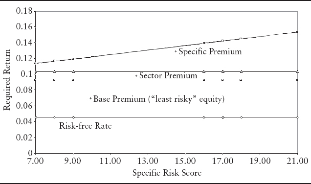
Here, the cost of equity is modeled in the context of four elements: (1) a risk-free rate of interest, (2) a base or nondiversifiable risk premium to the “least risky” equity, (3) a sector-risk premium, and (4) a company-specific risk premium related to (say) abnormal firm size, leverage (debt–equity ratio), and EVA volatility. While we make no specific recommendation, the investor or analyst needs to decide on a particular approach to measuring the cost of equity, as the required ROE is a key component of the WACC used in the EVA formulation. The required return is also a key ingredient in the residual income or abnormal earnings approach, which we describe next.

Cash-Flow Return on Investment

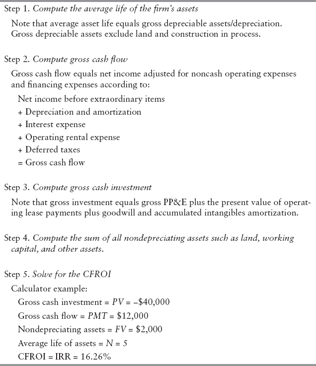
Another widely used VBM is the cash-flow return on investment (CFROI^®). CFROI is a commercial metric of Credit Suisse/HOLT. This metric is an internal rate of return (IRR)–based measure of company performance. CFROI takes on an economic profit perspective when it is compared to the cost of capital, WACC. Exhibit 2.8 shows a five-step process to calculate CFROI, although the actual calculation by CS/HOLT is much more complex with several value-based accounting adjustments. The exhibit also shows a simple example of how to estimate this widely known metric.

In Exhibit 2.8, the estimated CFROI is 16.26%. As a stand-alone figure, CFROI does not give the investor or analyst any indication of whether a company is pointing in the direction of wealth creation or destruction. However, CFROI takes on an economic profit perspective when the estimated IRR is compared to the cost of capital. Moreover, an economic profit relationship exists between the two VBMs because the spread between CFROI and WACC is similar to the economic profit or EVA spread.

Specifically, we know that EVA can be expressed in two ways:

Or, in spread form,

In principle, ROC is similar to CFROI, which is an IRR or rate of return on capital concept. While in theory the two value-based metrics (EVA and CFROI) are related in concept, there are notable differences in how these metrics are calculated in practice. A closer look at EVA and CFROI reveals that:

• EVA is a dollar-based measure of economic profit. CFROI is an IRR-like measure that takes on an economic profit perspective when compared to WACC.
• EVA uses NOPAT and net invested capital, while CFROI is based on gross cash flows and gross investment.
• EVA is measured in nominal terms, while CFROI is measured in real terms.
• The accounting adjustments used to measure EVA and CFROI may differ in practice.

EXHIBIT 2.8 CFROI: A Five-Step Process to Calculate CFROI

Residual Income

Another popular value-based metric is residual income (RI) or abnormal earnings. Residual income is simply accounting net income less the dollar cost of equity:

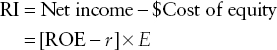
In this expression, the difference between ROE and the investor's required return (r) is the residual income (abnormal earnings) spread. While RI is analogous to EVA in that the measure of profit is net of the investor's dollar-based required return, the concept is somewhat less robust than EVA because ROE in the traditional realm of financial analysis reflects a mixing of operating and financing decisions.

Recall that in the Dupont formula ROE can be expressed as ROA times the equity multiplier (A/E). In contrast, in the EVA calculation the firm's operating and financing decisions are analyzed separately via NOPAT and $WACC. On the other hand, given the different reporting classifications on income and balance sheets for financial services versus nonfinancial services companies (e.g., loans are an asset for a bank while a liability for an industrial or technology firm), the RI (abnormal earnings) approach to equity analysis—with its focus on adjusted book value and the residual income spread—is particularly helpful in estimating and valuing the economic earnings of financial services companies.

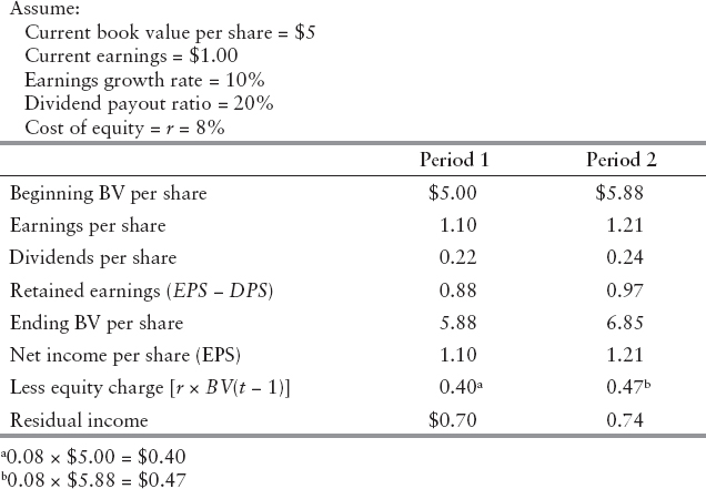
Exhibit 2.9 provides an example of how to calculate expected future values of RI given (1) the current book value, (2) a consensus earnings growth estimate, (3) an assumed dividend payout ratio (or implied plowback ratio), and (4) the cost of equity.

Since the RI estimates in Exhibit 2.8 are positive, at $0.70 and $0.74 per share, the firm is expected to make a value-added contribution to shareholder equity. This happens because the estimated ROE (EPS/BV) figures for periods 1 and 2, at 22% and 20.58%, are higher than the investor's assumed required return of 8%.

Role of EVA Momentum

We now describe how the concept of EVA momentum (and, by extension, residual income or abnormal earnings momentum) can be used as a prism to discern good company growth characteristics from bad company growth characteristics. While the level of EVA is important in deciding whether a company is a value creator or value destroyer, this information may already be reflected in share price. Hence, investors need to assess whether the level of EVA is increasing or decreasing. A firm's EVA momentum can be assessed according to

EXHIBIT 2.9 Forecasting Residual Income

With EVA spread constancy, we see that the change in EVA is driven by the change in net invested capital; that is, capital investment beyond depreciation. We illustrate the importance of EVA momentum by placing companies into four quadrants. The EVA quadrants (or EVA “style”) approach to equity analysis was developed by Grant and Abate⁴ and applied in Abate, Grant, and Stewart⁵ and Grant and Trahan.⁶ As shown in Exhibit 2.10, the EVA quadrants are defined by the following characteristics:

• Quadrant 1: Stagnant company—ROC > WACC; ΔC ≤ 0
• Quadrant 2: Good company growth—ROC > WACC; ΔC > 0
• Quadrant 3: Bad company growth—ROC < WACC; ΔC > 0
• Quadrant 4: Positive Restructure—ROC < WACC; ΔC < 0

We apply this schematic to S&P Industrial stocks. In Exhibit 2.10, Quadrant 2 and 4 companies have positive EVA momentum. In contrast, Quadrant 1 and 3 companies are for differing reasons destroying economic value added. This is because the stagnant/mature companies in Quadrant 1 have limited future growth opportunities, while Quadrant 3 companies are expanding negative EVA spread businesses. Clearly, Quadrant 2 and 4 companies represent potential buy opportunities, while companies that populate Quadrants 1 and 3 are potential sell or short-sell candidates, assuming that market implied expectations of future EVA growth are not fully reflected in share price (see EVA valuation considerations in the next section). Grant and Abate emphasize the EVA spread and capital expansion term (or capital catalyst) in the screening of good companies from bad or risky-troubled companies.

Valuation Considerations

We now describe how to use EVA valuation concepts to identify potential buy opportunities (those we refer to as good stocks) and sell or short sell opportunities (those we identify as bad stocks). To illustrate the diversity of valuation approaches using VBM concepts, we also show how to estimate the intrinsic value of a share of common stock using the residual income or abnormal earnings valuation model. RI valuation is similar to EVA valuation, with the substitution of residual income for EVA, and the residual income (abnormal earnings) spread for the EVA spread.

EXHIBIT 2.10 EVA Spread vs. Capital Growth: S&P Industrials

Identifying Good Stocks

While EVA momentum can be used to distinguish good companies from bad companies, we still must see whether a stock is a potential buy or sell opportunity. That is, if the market is efficient, then market implied expectations of future economic profit growth will be consistent with actual growth expectations that a company can deliver. In this case, the stock would be fairly priced in the marketplace. However, if actual expectations of future economic profit growth are higher than market implied expectations, then a stock would be considered undervalued. In turn, if actual expectations of future EVA growth are lower than that embedded in share price, then a stock would be overvalued.

In theory, it can be shown that a firm's net present value (NPV) is equal to the present value of all future EVA. With constant growth, the firm's NPV—a measure of intrinsic value added in current dollars—can be expressed as

In this expression, EVA is a one-step-ahead forecast, WACC is the familiar cost of capital, and g is the expected long-run growth in economic earnings. Of course, this form of EVA valuation requires that WACC is greater than the growth rate. It follows that the intrinsic value of the firm can be expressed as:

From these relationships, we can calculate the value–capital ratio (V/C). This ratio is analogous to the price–book value ratio in the traditional realm of financial analysis:

Since NPV (derived from EVA valuation) measures the value that a firm's management has added (albeit market and industry considerations) to the invested capital in their employ, the value–capital ratio is greater than unity if and only if the firm has discounted positive EVA; that is, NPV is positive, signifying a wealth creator. Equivalently, the V/C ratio is greater than one if the firm's management can sustainably generate a positive EVA spread [ROC > WACC, and WACC > g in the constant growth EVA valuation model].

In contrast, a firm's V/C ratio will be less than unity if discounted EVA is negative [ROC < WACC]; that is, NPV is negative, signifying a wealth destroyer. Note, too, that if the capital market is efficient, then the market's assessment of value added, denoted by MVA, will be equal to the firm's assessed NPV. From these relationships, we can identify the value-based conditions for discovering fairly priced stocks, undervalued stocks, and overvalued stocks; whereby MVA is equal to NPV, MVA is less than NPV, or MVA is higher than NPV, respectively. We summarize the security selection implications of these MVA and NPV conditions as:

Relationship	Condition
MVA = NPV	Stock is fairly priced
MVA < NPV	Stock is undervalued
MVA > NPV	Stock is overvalued

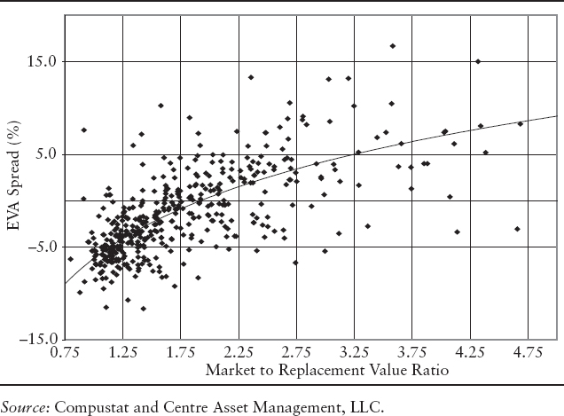
Exhibit 2.11 provides a graphical display of the EVA spread versus the V/C ratio for S&P Industrial stocks. The graph in this exhibit follows the EVA quadrants graph shown in Exhibit 2.10, and is based on the EVA style of investing approach developed by Grant and Abate.⁷

In Exhibit 2.11, the EVA spread is the y variable, while the V/C ratio is the x variable. Stocks that plot above the curve are deemed undervalued or good stocks as actual expectations of future economic profit growth, g, are higher than that reflected in share price; hence, the V/C ratio and stock price should rise. Stocks that plot below the curve are deemed overvalued or bad stocks since actual expectations of economic profit growth are lower than that embedded in share price; hence, V/C ratio and stock price should fall. In turn, stocks that plot on the curve are presumed to be efficiently priced as market implied expectations of future economic profit growth are equal to that which a company can realistically deliver. Moreover, a residual income (abnormal earnings) version of this EVA framework would show the residual income spread (ROE minus r) as the y variable and the price/book value ratio as the x variable.

EXHIBIT 2.11 EVA Spread vs. Value/Capital Ratio: S&P Industrials

Residual Income (Abnormal Earnings) Valuation

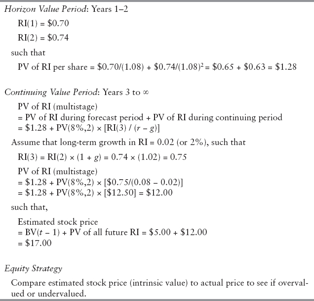
We now illustrate how to calculate the intrinsic value of a share of stock using the residual income or abnormal earnings model. Specifically, Exhibit 2.12 shows how to calculate the intrinsic value of a share of common stock using a two-stage (or multistage) RI model. The valuation analysis assumes a required return (cost of equity) of 8%, along with forecasted EPS over a finite horizon period (we use the two years of RI estimates from Exhibit 2.8) and forecasted continuing residual earnings.

Like EVA, we can explain the relationship between residual income and the justified price–book ratio based on forecasted fundamentals. Since the forecasted fundamentals approach to multiples analysis is a discounted cash flow (DCF) or intrinsic value approach, we have

such that

EXHIBIT 2.12 Residual Income Valuation

where P/BV > 1.0 if the present value of residual income (abnormal earnings) is positive. In contrast, P/BV is less than unity when a company is perceived to have consistently negative residual income. Equivalently, P/BV ratio is greater than one if ROE is sustainably greater than r, while P/BV is less than unity when the firm is perceived to incur a negative residual income spread [ROE < r].

Moreover, we could calculate the implied growth rate in residual income given the price–book ratio and an estimate of the required rate of return on equity. Using the constant growth assumption yields,

such that P/BV = 1 + [ROE – r]/(r – g).

Hence, the investor or analyst could solve for market-implied growth in residual income, g, with knowledge of P/BV, ROE, and the investor's required rate of return. The investor could then compare market-implied g with the long-term growth in residual income that the analyst perceives the company could actually deliver to determine whether a stock is a potential buy or sell opportunity.

VBM Caveats

While value-based metrics such as EVA, CFROI, and RI are fundamentally linked to value creation (via NPV), there are numerous accounting adjustments that an investor or analyst must consider in practice. Indeed, the firm of Stern Stewart has discovered some 140 accounting adjustments to consider when moving from the traditional accounting concept of income to the VBM concept of economic earnings. At a minimum, we recommend that investors and analysts consider the following list of VBM accounting adjustments when measuring economic profit:

• Research and development (capitalized)
• Strategic investments (temporary suspension of capital charge)
• Intangibles (capitalized and not amortized)
• Deferred taxes (conversion to cash taxes)
• Operating leases (treated as debt equivalent)
• Last in, first out (LIFO) inventory costing-LIFO reserve add backs

It is important to note that there are income statement and balance sheet consequences for each VBM accounting adjustment. For instance, the year-over-year change in an unamortized research and development (R&D) account (that is, amortization expense) would get added back to NOPAT, while the accumulated unamortized R&D account would get added back to EVA capital. In this way, the capitalized value of each dollar of R&D has a capital cost as long as it remains on the EVA balance sheet. Also, the after-tax implied interest expense on operating leases would get added back to NOPAT, while the present value of operating leases would be treated as a debt equivalent on the EVA balance sheet. VBM accounting conventions apply to several other value-based accounting items.

Despite the caveats or limitations cited for both traditional and value-based approaches to equity analysis, we conclude this chapter by recommending that investors join the two approaches to securities analysis. In the process, investors and analysts must realize that a combination of traditional and VBM analyses will require an extra effort in terms of the acquisition of knowledge and skills in order to understand what these metrics have to say about the creation of shareholder value. That being said, we believe that the extra time spent will be worth the effort in terms of both educational value added and economic value added—a doubly winning EVA benefit!

Case Study: JLG Equity Analysis Template

We present in the appendix to this chapter a synthesized traditional and value-based analysis of Coca-Cola using financial software developed by JLG Research. The accompanying equity analysis includes growth rates, margins, multiples, ROE, and FSR on the traditional side and EVA, EVA spread, residual income (abnormal earnings), and EVA momentum on the value-based metrics side. The equity analysis template shown herewith can be used to distinguish good companies (potential buy opportunities) from average to risky-troubled companies (potential sell or short sell opportunities). The data inputs for the JLG Equity Analysis Template are drawn from a Value Line report.

We emphasize that the case study application is not meant to show that traditional metrics are better or worse than VBM, or that our stock recommendation is somehow better than that provided by Value Line. Rather, the goal of the case study application of Coca-Cola is to show that traditional and VBM analyses can in fact complement each other; noting that we give Coca-Cola a “Timeliness” rating of “2” and a “Safety” rating of unity. Based on the Value Line scaling of 1 to 5, these fundamental ratings represent high expected performance over the next 6 to 12 months and low expected risk (from the date of the analysis). Incidentally, Value Line gave the soft-drink company a Timeliness rating of “3” for average expected performance over the forward 6 to 12 months with their highest safety rating as of the report date. With respect to these comparative ratings, we realize that past performance is no guarantee of future performance and that investors should seek professional advice when buying or selling securities.