GENERAL MODELS

Let us generalize the idea of statistical arbitrage. Imagine that there are two price processes (realistic processes will be stochastic), A(t, x_t, z_z) and B(t, y_t, z_z). The arguments can be thought of as time (t), a unique factor to A and B (x and y, respectively), and a common factor (z). If you let w_A,t and w_B,t represent the number of shares invested in each, and these numbers need not be constant, then a statistical arbitrage opportunity exists if there is a zero cost position that never (i.e., for all t) becomes negative.

The initial position, at time zero, is given by w_A,0A(0,x₀,z₀) + w_B,0B(0,y₀,z₀). This must be equal to zero in order to be a zero cost position to establish.

At any time after the position has been established, the value of the position must be greater than or equal to zero, represented by w_A,tA(t,x_t,z_t) + w_B,tB(t,y_t,z_t).

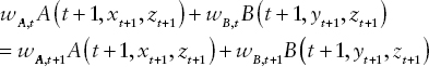
The portfolio positions, w_A,t and w_B,t, evolve according to the relationship that the strategy is “self-funding,” or “self-financing.” This simply means that when a position is established at time t, the portfolio is adjusted at t + 1 only with the proceeds from having held the portfolio positions from time t. This can be represented by the equation

At the terminal time, T, the portfolio value must be greater than zero to yield a profit, . The reason we use w_A,T−1and w_B,T−1 in the terminal portfolio value is that the position is established at time T−1 and held to time T.

One can think of the preceding as a system of equations where the weights need to be found such that initially it costs nothing to establish the position, there is never a possibility of a margin call (the portfolio's value must always be nonnegative), and on the terminal date the portfolio's value is strictly positive. There is also the constraint that the trading strategy must be self-financing, with the weights not having intraperiod changes: The weights are chosen at the beginning of the period and the value of the portfolio at the end of one period must be the same as the value of the portfolio at the beginning of the next period.

The preceding describes a dynamic programming problem. The objective function can be to maximize the terminal value of the portfolio, denoted by , where one selects the two sequences and .

If the price processes are stochastic, then this becomes a stochastic, dynamic programming problem subject to an informational constraint where we try to maximize the expected value of the portfolio at time T with only knowledge up to the present (t < T). The decision variables are the weights at each time step from t = 0 to t = T – 1.

The preceding is the general framework. Everything beyond that is a special case of the preceding: what are the unique and common factors, what are the models of the price processes, and are the weights constants or can they vary? Specific implementation requires modeling the price processes. So we are back where we started—the biggest risk in statistical arbitrage is model risk: Does the model of the price process comport to reality and will it persist over the investment horizon?