FACTOR MODELS

Classical financial theory states that the average return of a stock is the payoff to investors for taking on risk. One way of expressing this risk-reward relationship is through a factor model. A factor model can be used to decompose the returns of a security into factor-specific and asset-specific returns,

where β_i,1, β_i,2, …, β_i,K are the factor exposures of stock i, f_1,t, f_2,t, …, f_K,t are the factor returns, α_i is the average abnormal return of stock i, and _i,t is the residual.

This factor model specification is contemporaneous, that is, both left- and right-hand side variables (returns and factors) have the same time subscript, t. For trading strategies one generally applies a forecasting specification where the time subscript of the return and the factors are t + h (h ≥ 1) and t, respectively. In this case, the econometric specification becomes

How do we interpret a trading strategy based on a factor model? The explanatory variables represent different factors that forecast security returns, each factor has an associated factor premium. Therefore, future security returns are proportional to the stock's exposure to the factor premium,

and the variance of future stock return is given by

where and .

In the next section we discuss some specific econometric issues regarding cross-sectional regressions and factor models.

Econometric Considerations for Cross-Sectional Factor Models

In cross-sectional regressions, where the dependent variable⁴ is a stock's return and the independent variables are factors, inference problems may arise that are the result of violations of classical linear regression theory. The three most common problems are measurement problems, common variations in residuals, and multicollinearity.

Measurement Problems

Some factors are not explicitly given, but need to be estimated. These factors are estimated with an error. This error can have an impact on the inference from a factor model. This problem is commonly referred to as the “errors in variables problem.” For example, a factor that is comprised of a stock's beta is estimated with an error because beta is determined from a regression of stock excess returns on the excess returns of a market index. While beyond the scope of this book, several approaches have been suggested to deal with this problem.⁵

Common Variation in Residuals

The residuals from a regression often contain a source of common variation. Sources of common variation in the residuals are heteroskedasticity and serial correlation.⁶ We note that when the form of heteroskedasticity and serial correlation is known, we can apply generalized least squares (GLS). If the form is not known, it has to be estimated, for example as part of feasible generalized least squares (FGLS). We summarize some additional possibilities next.

Heteroskedasticity occurs when the variance of the residual differs across observations and affects the statistical inference in a linear regression. In particular, the estimated standard errors will be underestimated and the t-statistics will therefore be inflated. Ignoring heteroskedasticity may lead the researcher to find significant relationships where none actually exist. Several procedures have been developed to calculate standard errors that are robust to heteroskedasticity, also known as heteroskedasticity-consistent standard errors.

Serial correlation occurs when residuals terms in a linear regression are correlated, violating the assumptions of regression theory. If the serial correlation is positive, then the standard errors are underestimated and the t-statistics will be inflated. Cochrane⁷ suggests that the errors in cross-sectional regressions using financial data are often off by a factor of 10. Procedures are available to correct for serial correlation when calculating standard errors.

When the residuals from a regression are both heteroskedastic and serially correlated, procedures are available to correct them. One commonly used procedure is the one proposed by Newey and West referred to as the “Newey-West corrections,”⁸ and its extension by Andrews.⁹

Petersen¹⁰ provides guidance on choosing the appropriate method to use for correctly calculating standard errors in panel data regressions when the residuals are correlated. He shows the relative accuracy of the different methods depends on the structure of the data. In the presence of firm effects, where the residuals of a given firm may be correlated across years, ordinary least squares (OLS), Newey-West (modified for panel data sets), or Fama-MacBeth,¹¹ corrected for first-order autocorrelation, all produce biased standard errors. To correct for this, Petersen recommends using standard errors clustered by firms. If the firm effect is permanent, the fixed effects and random effects models produce unbiased standard errors. In the presence of time effects, where the residuals of a given period may be correlated across difference firms (cross-sectional dependence), Fama-MacBeth produces unbiased standard errors. Furthermore, standard errors clustered by time are unbiased when there are a sufficient number of clusters. To select the correct approach he recommends determining the form of dependence in the data and comparing the results from several methods.

Gow, Ormazabal, and Taylor¹² evaluate empirical methods used in accounting research to correct for cross-sectional and time-series dependence. They review each of the methods, including several methods from the accounting literature that have not previously been formally evaluated, and discuss when each methods produces valid inferences.

Multicollinearity

Multicollinearity occurs when two or more independent variables are highly correlated. We may encounter several problems when this happens. First, it is difficult to determine which factors influence the dependent variable. Second, the individual p values can be misleading—a p value can be high even if the variable is important. Third, the confidence intervals for the regression coefficients will be wide. They may even include zero. This implies that, we cannot determine whether an increase in the independent variable is associated with an increase—or a decrease—in the dependent variable. There is no formal solution based on theory to correct for multicollinearity. The best way to correct for multicollinearity is by removing one or more of the correlated independent variables. It can also be reduced by increasing the sample size.

Fama-MacBeth Regression

To address the inference problem caused by the correlation of the residuals, Fama and MacBeth¹³ proposed the following methodology for estimating cross-sectional regressions of returns on factors. For notational simplicity, we describe the procedure for one factor. The multifactor generalization is straightforward.

First, for each point in time t we perform a cross-sectional regression:

In the academic literature, the regressions are typically performed using monthly or quarterly data, but the procedure could be used at any frequency.

The mean and standard errors of the time series of slopes and residuals are evaluated to determine the significance of the cross-sectional regression. We estimate f and _i as the average of their cross-sectional estimates, therefore,

The variations in the estimates determine the standard error and capture the effects of residual correlation without actually estimating the correlations.¹⁴ We use the standard deviations of the cross-sectional regression estimates to calculate the sampling errors for these estimates,

Cochrane¹⁵ provides a detailed analysis of this procedure and compares it to cross-sectional OLS and pooled time-series cross-sectional OLS. He shows that when the factors do not vary over time and the residuals are cross-sectionally correlated, but not correlated over time, then these procedures are all equivalent.

Information Coefficients

To determine the forecast ability of a model, practitioners commonly use a statistics called the information coefficient (IC). The IC is a linear statistic that measures the cross-sectional correlation between a factor and its subsequent realized return:¹⁶

where f_t is a vector of cross sectional factor values at time t and r_t,t+k is a vector of returns over the time period t to t + k.

Just like the standard correlation coefficient, the values of the IC range from −1 to +1. A positive IC indicates a positive relation between the factor and return. A negative IC indicates a negative relation between the factor and return. ICs are usually calculated over an interval, for example, daily or monthly. We can evaluate how a factor has performed by examining the time series behavior of the ICs. Looking at the mean IC tells how predictive the factor has been over time.

An alternate specification of this measure is to make f_t the rank of a cross-sectional factor. This calculation is similar to the Spearman rank coefficient. By using the rank of the factor, we focus on the ordering of the factor instead of its value. Ranking the factor value reduces the unduly influence of outliers and reduces the influence of variables with unequal variances. For the same reasons, we may also choose to rank the returns instead of using their numerical value.

Sorensen, Qian, and Hua¹⁷ present a framework for factor analysis based on ICs. Their measure of IC is the correlation between the factor ranks, where the ranks are the normalized z-score of the factor,¹⁸ and subsequent return. Intuitively, this IC calculation measures the return associated with a one standard deviation exposure to the factor. Their IC calculation is further refined by risk adjusting the value. To risk adjust, the authors remove systematic risks from the IC and accommodate the IC for specific risk. By removing these risks, Qian and Hua¹⁹ show that the resulting ICs provide a more accurate measure of the return forecasting ability of the factor.

The subsequent realized returns to a factor typically vary over different time horizons. For example, the return to a factor based on price reversal is realized over short horizons, while valuation metrics such as EBITDA/EV are realized over longer periods. It therefore makes sense to calculate multiple ICs for a set of factor forecasts whereby each calculation varies the horizon over which the returns are measured.

The IC methodology has many of the same advantages as regression models. The procedure is easy to implement. The functional relationship between factor and subsequent returns is known (linear).

ICs can also be used to assess the risk of factors and trading strategies. The standard deviation of the time series (with respect to t) of ICs for a particular factor (std(IC_t,t+k)) can be interpreted as the strategy risk of a factor. Examining the time series behavior of std(IC_t,t+k) over different time periods may give a better understanding of how often a particular factor may fail. Qian and Hua show that std(IC_t,t+k) can be used to more effectively understand the active risk of investment portfolios. Their research demonstrates that ex post tracking error often exceeds the ex ante tracking provided by risk models. The difference in tracking error occurs because tracking error is a function of both ex ante tracking error from a risk model and the variability of information coefficients, std(IC_t,t+k). They define the expected tracking error as

where N is the number of stocks in the universe (breath), σ_model is the risk model tracking error, and dis(R_t) is dispersion of returns²⁰ defined by

Example: Information Coefficients

Exhibit 12.4 displays the time-varying behavior of ICs for each one of the factors EBITDA/EV, growth of fiscal year 1 and fiscal year 2 earnings estimates, revisions, and momentum. The graph shows the time series average of information coefficients:

The graph depicts the information horizons for each factor, showing how subsequent return is realized over time. The vertical axis shows the size of the average information coefficient for k = 1, 2, …, 15.

Specifically, the EBITDA/EV factor starts at almost 0.03 and monotonically increases as the investment horizon lengthens from one month to 15 months. At 15 months, the EBITDA/EV factor has an IC of 0.09, the highest value among all the factors presented in the graph. This relationship suggests that the EBITDA/EV factor earns higher returns as the holding period lengthens.

EXHIBIT 12.4 Information Coefficients over Various Horizons for EBITDA/EV, Growth of Fiscal Year 1 and Fiscal Year 2 Earnings Estimates, Revisions, and Momentum Factors

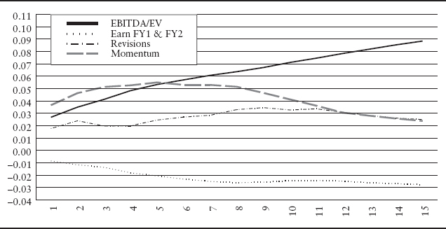
The other ICs of the factors in the graph are also interesting. The growth of fiscal year 1 and fiscal year 2 earnings estimates factor is defined as the growth in current fiscal year (fy1) earnings estimates to the next fiscal year (fy2) earnings estimates provided by sell-side analysts.²¹ We call the growth of fiscal year 1 and fiscal year 2 earnings estimates factor the earnings growth factor throughout the remainder of the chapter. The IC is negative and decreases as the investment horizon lengthens. The momentum factor starts with a positive IC of 0.02 and increases to approximately 0.055 in the fifth month. After the fifth month, the IC decreases. The revisions factor starts with a positive IC and increases slightly until approximately the eleventh month at which time the factor begins to decay.

Looking at the overall patterns in the graph, we see that the return realization pattern to different factors varies. One notable observation is that the returns to factors don't necessarily decay but sometimes grow with the holding period. Understanding the multiperiod effects of each factor is important when we want to combine several factors. This information may influence how one builds a model. For example, we can explicitly incorporate this information about information horizons into our model by using a function that describes the decay or growth of a factor as a parameter to be calibrated. Implicitly, we could incorporate this information by changing the holding period for a security traded for our trading strategy. Specifically, Sneddon²² discusses an example that combines one signal that has short-range predictive power with another that has long-range power. Incorporating this information about the information horizon often improves the return potential of a model. Kolm²³ describes a general multiperiod model that combines information decay, market impact costs, and real world constraints.

Factor Portfolios

Factor portfolios are constructed to measure the information content of a factor. The objective is to mimic the return behavior of a factor and minimize the residual risk. Similar to portfolio sorts, we evaluate the behavior of these factor portfolios to determine whether a factor earns a systematic premium.

Typically, a factor portfolio has a unit exposure to a factor and zero exposure to other factors. Construction of factor portfolios requires holding both long and short positions. We can also build a factor portfolio that has exposure to multiple attributes, such as beta, sectors, or other characteristics. For example, we could build a portfolio that has a unit exposure to book-to-price and small size stocks. Portfolios with exposures to multiple factors provide the opportunity to analyze the interaction of different factors.

A Factor Model Approach

By using a multifactor model, we can build factor portfolios that control for different risks.²⁴ We decompose return and risk at a point in time into a systematic and specific component using the regression:

where r is an N vector of excess returns of the stocks considered, X is an N by K matrix of factor loadings, b is a K vector of factor returns, and u is a N vector of firm specific returns (residual returns). Here, we assume that factor returns are uncorrelated with the firm specific return. Further assuming that firm specific returns of different companies are uncorrelated, the N by N covariance matrix of stock returns V is given by

where F is the K by K factor return covariance matrix and Δ is the N by N diagonal matrix of variances of the specific returns.

We can use the Fama-MacBeth procedure discussed earlier to estimate the factor returns over time. Each month, we perform a GLS regression to obtain

OLS would give us an unbiased estimate, but since the residuals are heteroskedastic the GLS methodology is preferred and will deliver a more efficient estimate. The resulting holdings for each factor portfolio are given by the rows of (X'Δ⁻¹X)⁻¹ XΔ⁻¹.

An Optimization-Based Approach

A second approach to build factor portfolios uses mean-variance optimization. Using optimization techniques provide a flexible approach for implementing additional objectives and constraints.²⁵

Using the notation from the previous subsection, we denote by X the set of factors. We would like to construct a portfolio that has maximum exposure to one target factor from X (the alpha factor), zero exposure to all other factors, and minimum portfolio risk. Let us denote the alpha factor by X_α and all the remaining ones by X_α. Then the resulting optimization problem takes the form

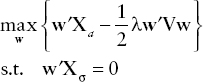
The analytical solution to this optimization problem is given by

We may want to add additional constraints to the problem. Constraints are added to make factor portfolios easier to implement and meet additional objectives. Some common constraints include limitations on turnover, transaction costs, the number of assets, and liquidity preferences. These constraints²⁶ are typically implemented as linear inequality constraints. When no analytical solution is available to solve the optimization with linear inequality constraints, we have to resort to quadratic programming (QP).²⁷