
BENCHMARK EXPOSURE AND TRACKING ERROR MINIMIZATION
Expected portfolio return maximization under the mean-variance framework or other risk measure minimization are examples of active investment strategies, that is, strategies that identify a universe of attractive investments, and ignore inferior investments opportunities. A different approach, referred to as a passive investment strategy, argues that in the absence of any superior forecasting ability, investors might as well resign themselves to the fact that they cannot beat the market. From a theoretical perspective, the analytics of portfolio theory tell them to hold a broadly diversified portfolio anyway. Many mutual funds are managed relative to a particular benchmark or stock universe, such as the S&P 500 or the Russell 1000. The portfolio allocation models are then formulated in such a way that the tracking error relative to the benchmark is kept small.
Standard Definition of Tracking Error
To incorporate a passive investment strategy, we can change the objective function of the portfolio allocation problem so that instead of minimizing a portfolio risk measure, we minimize the tracking error with respect to a benchmark that represents the market, such as the Russell 3000, or the S&P 500. Such strategies are often referred to as indexing. The tracking error can be defined in different ways. However, practitioners typically mean a specific definition: the variance (or standard deviation) of the difference between the portfolio return, ![]() , and the return on the benchmark,
, and the return on the benchmark, ![]() . Mathematically, the tracking error (TE) can be expressed as
. Mathematically, the tracking error (TE) can be expressed as
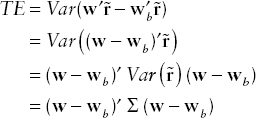
where Σ is the covariance matrix of the stock returns. One can observe that the formula is very similar to the formula for the portfolio variance; however, the portfolio weights in the formula for the variance are replaced by differences between the weights of the stocks in the portfolio and the weights of the stocks in the index.
Why do we need to optimize portfolio weights in order to track a benchmark, when technically the most effective way to track a benchmark is by investing the portfolio in the stocks in the benchmark portfolio in the same proportions as the proportions of these securities in the benchmark? The problem with this approach is that, especially with large benchmarks like the Russell 3000, the transaction costs of a proportional investment and the subsequent rebalancing of the portfolio can be prohibitive (that is, dramatically adversely impact the performance of the portfolio relative to the benchmark). Furthermore, in practice securities are not infinitely divisible, so investing a portfolio of a limited size in the same proportions as the composition of the benchmark will still not achieve zero tracking error. Thus, the optimal formulation is to require that the portfolio follows the benchmark as closely as possible.
While indexing has become an essential part of many portfolio strategies, most portfolio managers cannot resist the temptation to identify at least some securities that will outperform others. Hence, restrictions on the tracking error are often imposed as a constraint, while the objective function is something different than minimizing the tracking error. The tracking error constraint takes the form
![]()
where ![]() is a limit (imposed by the investor) on the amount of tracking error the investor is willing to tolerate. This is a quadratic constraint, which is convex and computationally tractable, but requires specialized optimization software.
is a limit (imposed by the investor) on the amount of tracking error the investor is willing to tolerate. This is a quadratic constraint, which is convex and computationally tractable, but requires specialized optimization software.
Alternative Ways of Defining Tracking Error
There are alternative ways in which tracking-error type constraints can be imposed. For example, we may require that the absolute deviations of the portfolio weights (w) from the index weights (wb) are less than or equal to a given vector array of upper bounds u:
![]()
where the absolute values |.| for the vector differences are taken componentwise, that is, for pairs of corresponding elements from the two vector arrays. These constraints can be stated as linear constraints by rewriting them as
Similarly, we can require that for stocks within a specific industry (whose indexes in the portfolio belong to a subset Ij of the investment universe I), the total tracking error is less than a given upper bound Uj:
![]()
Finally, tracking error can be expressed through risk measures other than the absolute deviations or the variance of the deviations from the benchmark. Rockafellar and Uryasev5 suggest using Conditional Value-at-Risk (CVaR)6 to manage the tracking error. (Using CVaR as a risk measure results in computationally tractable optimization formulations for portfolio allocation, as long as the data are presented in the form of scenarios.7) We provide below a formulation that is somewhat different from Rockafellar and Uryasev, but preserves the main idea.
Suppose that we are given S scenarios for the return of a benchmark portfolio (or an instrument we are trying to replicate), bs, s = 1, …, S. These scenarios can be generated by simulation, or taken from historical data. We also have N stocks with returns ![]() (i = 1, …, N, s = 1, …, S) in each scenario. The value of the portfolio in scenario s is
(i = 1, …, N, s = 1, …, S) in each scenario. The value of the portfolio in scenario s is
![]()
or, equivalently, (r(s))′w, where r(s) is the vector of returns for the N stocks in scenario s. Consider the differences between the return on the benchmark and the return on the portfolio,
![]()
If this difference is positive, we have a loss; if the difference is negative, we have a gain; both gains and losses are computed relative to the benchmark. Rationally, the portfolio manager should not worry about differences that are negative; the only cause for concern would be if the portfolio underperforms the benchmark, which would result in a positive difference. Thus, it is not necessarily to limit the variance of the deviations of the portfolio returns from the benchmark, which penalizes for positive and negative deviations equally. Instead, we can impose a limit on the amount of loss we are willing to tolerate in terms of the CVaR of the distribution of losses relative to the benchmark.
The tracking error constraint in terms of the CVaR can be stated as the following set of constraints:8
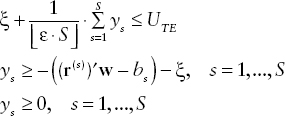
where UTE is the upper bound on the negative deviations.
This formulation of tracking error is appealing in two ways. First, it treats positive and negative deviations relative to the benchmark differently, which agrees with the strategy of an investor seeking to maximize returns overall. Second, it results in a linear set of constraints, which are easy to handle computationally, in contrast to the first formulation of the tracking error constraint in this section, which results in a quadratic constraint.
Actual vs. Predicted Tracking Error
The tracking error calculation in practice is often backward-looking. For example, in computing the covariance matrix Σ in the standard tracking error definition as the variance of the deviations of the portfolio returns from the index, or in selecting the scenarios used in the CVaR-type tracking error constraint in the previous section, we may use historical data. The tracking error calculated in this manner is called the ex post tracking error, backward-looking error, or actual tracking error.
The problem with using the actual tracking error for assessing future performance relative to a benchmark is that the actual tracking error does not reflect the effect of the portfolio manager's current decisions on the future active returns and hence the tracking error that may be realized in the future. The actual tracking error has little predictive value and can be misleading regarding portfolio risk.
Portfolio managers need forward-looking estimates of tracking error to reflect future portfolio performance more accurately. In practice, this is accomplished by using the services of a commercial vendor that has a multifactor risk model that has identified and defined the risks associated with the benchmark, or by building such a model in-house. Statistical analysis of historical return data for the stocks in the benchmark are used to obtain the risk factors and to quantify the risks. Using the manager's current portfolio holdings, the portfolio's current exposure to the various risk factors can be calculated and compared to the benchmark's exposures to the risk factors. From the differential factor exposures and the risks of the factors, a forward-looking tracking error for the portfolio can be computed. This tracking error is also referred to as ex ante tracking error or predicted tracking error.
There is no guarantee that the predicted tracking error will match exactly the tracking error realized over the future time period of interest. However, this calculation of the tracking error has its use in risk control and portfolio construction. By performing a simulation analysis on the factors that enter the calculation, the manager can evaluate the potential performance of portfolio strategies relative to the benchmark and eliminate those that result in tracking errors beyond the client-imposed tolerance for risk. The actual tracking error, on the other hand, is useful for assessing actual performance relative to a benchmark.