MARKET IMPACT MEASUREMENTS AND EMPIRICAL FINDINGS

The problem with measuring implicit transaction costs is that the true measure, which is the difference between the price of the stock in the absence of a money manager's trade and the execution price, is not observable. Furthermore, the execution price is dependent on supply and demand conditions at the margin. Thus, the execution price may be influenced by competitive traders who demand immediate execution or by other investors with similar motives for trading. This means that the execution price realized by an investor is the consequence of the structure of the market mechanism, the demand for liquidity by the marginal investor, and the competitive forces of investors with similar motivations for trading.

There are many ways to measure transaction costs. However, in general this cost is the difference between the execution price and some appropriate benchmark, a so-called fair market benchmark. The fair market benchmark of a security is the price that would have prevailed had the trade not taken place, the no-trade price. Since the no-trade price is not observable, it has to be estimated. Practitioners have identified three different basic approaches to measure the market impact:⁹

1. Pre-trade measures use prices occurring before or at the decision to trade as the benchmark, such as the opening price on the same-day or the closing price on the previous day.
2. Post-trade measures use prices occurring after the decision to trade as the benchmark, such as the closing price of the trading day or the opening price on the next day.
3. Same-day or average measures use average prices of a large number of trades during the day of the decision to trade, such as the volume-weighted average price (VWAP) calculated over all transactions in the security on the trade day.¹⁰

The volume-weighted average price is calculated as follows. Suppose that it was a trader's objective to purchase 10,000 shares of stock XYZ. After completion of the trade, the trade sheet showed that 4,000 shares were purchased at $80, another 4,000 at $81, and finally 2,000 at $82. In this case, the resulting VWAP is (4,000 × 80 + 4,000 × 81 + 2,000 × 82)/10,000 = $80.80.

We denote by χ the indicator function that takes on the value 1 or −1 if an order is a buy or sell order, respectively. Formally, we now express the three types of measures of market impact (MI) as follows

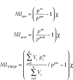
where p^ex, p^pre, and p^post denote the execution price, pre-trade price, and post-trade price of the stock, and k denotes the number of transactions in a particular security on the trade date. Using this definition, for a stock with market impact MI the resulting market impact cost for a trade of size V, MIC, is given by

It is also common to adjust market impact for general market movements. For example, the pre-trade market impact with market adjustment would take the form

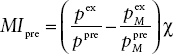
where represent the value of the index at the time of the execution, and the price of the index at the time before the trade. Market adjusted market impact for the post-trade and same-day trade benchmarks are calculated in an analogous fashion.

The above three approaches to measure market impact are based upon measuring the fair market benchmark of stock at a point in time. Clearly, different definitions of market impact lead to different results. Which one should be used is a matter of preference and is dependent on the application at hand. For example, Elkins and McSherry, a financial consulting firm that provides customized trading costs and execution analysis, calculates a same-day benchmark price for each stock by taking the mean of the day's open, close, high, and low prices. The market impact is then computed as the percentage difference between the transaction price and this benchmark. However, in most cases VWAP and the Elkins McSherry approach lead to similar measurements.¹¹

As we analyze a portfolio's return over time an important question to ask is whether we can attribute good/bad performance to investment profits/losses or to trading profits/losses. In other words, in order to better understand a portfolio's performance it can be useful to decompose investment decisions from order execution. This is the basic idea behind the implementation shortfall approach.¹²

In the implementation shortfall approach, we assume that there is a separation between investment and trading decisions. The portfolio manager makes decisions with respect to the investment strategy (i.e., what should be bought, sold, and held). Subsequently, these decisions are implemented by the traders.

By comparing the actual portfolio profit/loss (P/L) with the performance of a hypothetical paper portfolio in which all trades are made at hypothetical market prices, we can get an estimate of the implementation shortfall. For example, with a paper portfolio return of 6% and an actual portfolio return of 5%, the implementation shortfall is 1%.

There is considerable practical and academic interest in the measurement and analysis of international trading costs. Domowitz, Glen, and Madhavan¹³ examine international equity trading costs across a broad sample of 42 countries using quarterly data from 1995 to 1998. They find that the mean total one-way trading cost is 69.81 basis points. However, there is an enormous variation in trading costs across countries. For example, in their study the highest was Korea with 196.85 basis points whereas the lowest was France with 29.85 basis points. Explicit costs are roughly two-thirds of total costs. However, one exception to this is the United States where the implicit costs are about 60% of the total costs.

Transaction costs in emerging markets are significantly higher than those in more developed markets. Domowitz, Glen, and Madhavan argue that this fact limits the gains of international diversification in these countries explaining in part the documented home bias of domestic investors.

In general, they find that transaction costs declined from the middle of 1997 to the end of 1998, with the exception of Eastern Europe. It is interesting to notice that this reduction in transaction costs happened despite the turmoil in the financial markets during this period. A few explanations that Domowitz et al. suggest are that (1) the increased institutional presence has resulted in a more competitive environment for brokers/dealers and other trading services; (2) technological innovation has led to a growth in the use of low-cost electronic crossing networks (ECNs) by institutional traders; and (3) soft dollar payments are now more common.