QUESTIONS

1. There are different ways of computing the expected shortfall of a portfolio. A common approach is to use historical asset returns to simulate the portfolio return distribution. In the study presented in this chapter, why did the authors use a factor model and the associated factor return history to simulate a portfolio's historical return distribution?
2. Discuss the difference between beta and shortfall beta.
3. By constraining shortfall beta, one tends to lower the standard beta of the portfolio, since the two are strongly correlated. Is the outperformance of shortfall constrained optimization for the findings reported in this chapter simply due to its lower beta, especially during the turbulent periods?
4. Does constraining shortfall help protect against sharp daily losses?
5. Can you provide any insight into why shortfall constrained optimization performed better than mean-variance optimization in the empirical study?

¹ Dimitris Bertsimas, Geoffrey J. Lauprete, and Alexander Samarov, “Shortfall as a Risk Measure: Properties, Optimization and Applications,” Journal of Economic Dynamics and Control 28, no. 7 (2004): 1353–1381.

² Lisa Goldberg, and Michael Hayes, “The Long View of Financial Risk,” report, MSCI Barra Research Insight (2009).

³ VaR can be computed at other likelihoods of loss as well. For example, The portfolio suffers a return worse than VaR_P at 1% or less no more than 1% of the time.

⁴ Lisa Goldberg, and Michael Hayes, “Barra Extreme Risk,” report, MSCI Barra Research Conference 2010.

⁵ MSCI Barra, Barra Extreme Risk Analytics Guide (New York: 2010).

⁶ Prior research has also shown how shortfall can be directly included in the objective function; see Bertsimas, Lauprete, and Samarov, “Shortfall as a Risk Measure: Properties, Optimization and Applications.” This approach deserves separate consideration, however, and we save this topic for a future study.

⁷ The decomposition shown in the paper is based on the portfolio optimality conditions. For the shortfall constrained problem, these conditions are

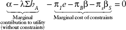
where h_A represents the active holdings and π_l, π_β, π_βs are the shadow prices of the full investment, beta and shortfall beta constraints, respectively. The shadow price of a constraint tells us how much utility changes as we increase the bound on the constraint. By multiplying both sides of the above equation by and rearranging terms, we can express the optimized portfolio's holdings as a sum of individual component portfolios as in equation (19.4). This is discussed further in Jennifer Bender, Jyh-Huei Lee, and Dan Stefek, “Decomposing the Impact of Portfolio Constraints,” MSCI Barra Research Insights (2009).

⁸ The shadow price of a constraint tells us how much utility changes as we increase the bound on the constraint.

⁹ Another way to scale factor returns is by the square root of the factor covariance matrix . In a separate study, we find that there is little difference between the results of this approach or from applying the Cholesky decomposition.

¹⁰ Another choice is to assume a distribution for the specific return and simulate scenarios from the distribution.