EQUITY RISK FACTOR MODELS

The design of a linear factor model usually starts with the identification of the major sources of risk embedded in the portfolios of interest. For an equity portfolio manager who invests in various markets across the globe, the major sources of risk are typically country, industry membership, and other fundamental or technical exposures such as size, value, and momentum. The relative significance of these components varies across different regions. For instance, for regional equity risk models in developed markets, industry factors tend to be more important than country factors, although in periods of financial distress country factors become more significant. On the other hand, for emerging markets models the country factor is still considered to be the most important source of risk. For regional models, the relative significance of industry factors depends on the level of financial integration across different local markets in that region. The importance of these factors is also time-varying, depending on the particular time period of the analysis. For instance, country risk used to be a large component of total risk for European equity portfolios. However, country factors have been losing their significance in this context due to financial integration in the region as a result of the European Union and a common currency, the euro. This is particularly true for larger European countries. Similarly, the relative importance of industry factors is higher over the course of certain industry-led crises, such as the dot-com bubble burst (2000–2002) and the 2007–2009 banking and credit crisis. As we will see, the relative importance of different risk factors varies also with the particular design and the estimation process chosen to calibrate the model.

A typical global or regional equity risk model has the following structure:

where

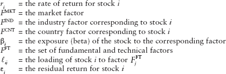
There are different ways in which these factors can be incorporated into an equity risk model. The choice of a particular model affects the interpretation of the factors. For instance, consider a model that has only market and industry factors. Industry factors in such a model would represent industry-specific moves net of the market return. On the other hand, if we remove the market factor from the equation, the industry factors now incorporate the overall market effect. Their interpretation would change, with their returns now being close to market value-weighted industry indexes. Country-specific risk models are a special case of the previous representation where the country factor disappears and the market factor is represented by the returns of the countrywide market. Macroeconomic factors are also used in some equity risk models, as discussed later.

The choice of estimation process also influences the interpretation of the factors. As an example, consider a model that has only industry and country factors. These factors can be estimated jointly in one step. In this case, both factors represent their own effect net of the other one. On the other hand, these factors can be estimated in a multistep process—e.g., industry factors estimated in the first step and then the country factors estimated in the second step, using residual returns from the first step. In this case, the industry factors have an interpretation close to the market value-weighted industry index returns, while the country factors would now represent a residual country average effect, net of industry returns. We discuss this issue in more detail in the following section.

Model Estimation

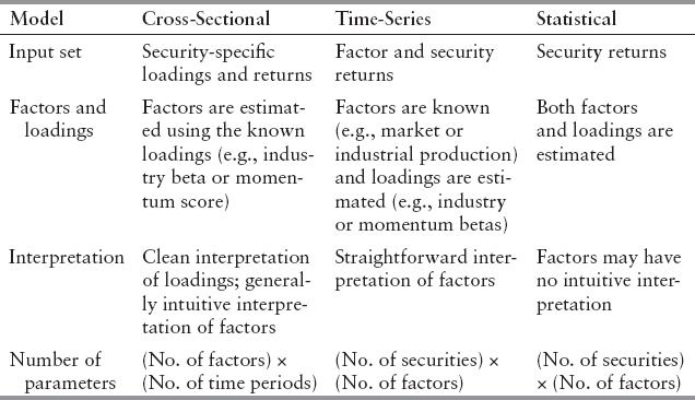
In terms of the estimation methodology, there are three major types of multi-factor equity risk models: cross-sectional, time series, and statistical. All three of these methodologies are widely used to construct linear factor models in the equity space.⁴ In cross-sectional models, loadings are known and factors are estimated. Examples of loadings used in these models are industry membership variables and fundamental security characteristics (e.g., the book-to-price ratio). Individual stock returns are regressed against these security-level loadings in every period, delivering estimation of factor returns for that period. The interpretation of these estimated factors is usually intuitive, although dependent on the estimation procedure and on the quality of the loadings. In time-series models, factors are known and loadings are estimated. Examples of factors in these models are financial or macroeconomic variables, such as market returns or industrial production. Time series of individual equity returns are regressed against the factor returns, delivering empirical sensitivities (loadings or betas) of each stock to the risk factors. In these models, factors are constructed and not estimated, therefore, their interpretation is straightforward. In statistical models (e.g., principal component analysis), both factors and loadings are estimated jointly in an iterative fashion. The resulting factors are statistical in nature, not designed to be intuitive. That being said, a small set of the statistical factors can be (and usually are) correlated with broad economic factors, such as the market. Exhibit 13.1 summarizes some of the characteristics of these models.

An important advantage of cross-sectional models is that the number of parameters to be estimated is generally significantly smaller as compared to the other two types of models. On the other hand, cross-sectional models require a much larger set of input data (company-specific loadings). Cross-sectional models tend to be relatively more responsive as loadings can adjust faster to changing market conditions. There are also hybrid models, which combine cross-sectional and time-series estimation in an iterative fashion; these models allow the combination of observed and estimated factors. Statistical models on the other hand require only a history of security returns as input to the process. They tend to work better when economic sources of risk are hard to identify and are primarily used in high-frequency applications.

EXHIBIT 13.1 Cross-Sectional, Time-Series, and Statistical Factor Models

As we mentioned in the previous section, the estimation process is a major determinant in the interpretation of factors. Estimating all factors jointly in one-step regression allows for a natural decomposition of total variance in stock returns. However it also complicates the interpretation of factors as each factor now represents its own effect net of all other factors. Moreover, multicollinearity problems arise naturally in this set-up, potentially delivering lack of robustness to the estimation procedure and leading to unintuitive factor realizations. This problem can be serious when using factors that are highly correlated.

An alternative in this case is to use a multistep estimation process where different sets of factors are estimated sequentially, in separate regressions. In the first step, stock returns are used in a regression to estimate a certain set of factors and then residual returns from this step are used to estimate the second step factors and so on. The choice of the order of factors in such estimation influences the nature of the factors and their realizations. This choice should be guided by the significance and the desired interpretation of the resulting factors. The first-step factors have the most straightforward interpretation as they are estimated in isolation from all other factors using raw stock returns. For instance in a country-specific equity risk model where there are only industry and fundamental or technical factors, the return series of industry factors would be close to the industry index returns if they are estimated in isolation in the first step. This would not be the case if all industry, fundamental, and technical factors are estimated in the same step.

An important input to the model estimation is the security weights used in the regressions. There is a variety of techniques employed in practice but generally more weight is assigned to less volatile stocks (usually represented by larger companies). This enhances the robustness of the factor estimates as stocks from these companies tend to have relatively more stable return distributions.

Types of Factors

In this section, we analyze in more detail the different types of factors typically used in equity risk models. These can be classified under five major categories: market factors, classification variables, firm characteristics, macroeconomic variables, and statistical factors.

Market Factors

A market factor can be used as an observed factor in a time-series setting (e.g., in the capital asset pricing model, the market factor is the only systematic factor driving returns). As an example, for a U.S. equity factor model, S&P 500 can be used as a market factor and the loading to this factor—market beta—can be estimated by regressing individual stock returns to the S&P 500. On the other hand, in a cross-sectional setting, the market factor can be estimated by regressing stock returns to the market beta for each time period (this beta can be empirical—estimated via statistical techniques—or set as a dummy loading, usually 1). When incorporated into a cross-sectional regression with other factors, it generally works as an intercept, capturing the broad average return for that period. This changes the interpretation of all other factors to returns relative to that average (e.g. industry factor returns would now represent industry-specific moves net of market).

Classification Variables

Industry and country are the most widely used classification variables in equity risk models. They can be used as observed factors in time-series models via country/industry indexes (e.g. return series of GICS indexes⁵ can be used as observed industry factors). In a cross-sectional setting, these factors are estimated by regressing stock returns to industry/country betas (either estimated or represented as a 0/1 dummy loading). These factors constitute a significant part of total risk for a majority of equity portfolios, especially for portfolios tilted toward specific industries or countries.

Firm Characteristics

Factors that represent firm characteristics can be classified as either fundamental or technical factors. These factors are extensively used in equity risk models; exposures to these factors represent tilts towards major investment themes such as size, value, and momentum. Fundamental factors generally employ a mix of accounting and market variables (e.g., accounting ratios) and technical factors commonly use return and volume data (e.g., price momentum or average daily volume traded).

In a time-series setting, these factors can be constructed as representative long-short portfolios (e.g., Fama-French factors). As an example, the value factor can be constructed by taking a long position in stocks that have a large book to price ratio and a short position in the stocks that have a small book to price ratio. On the other hand, in a cross-sectional setup, these factors can be estimated by regressing the stock returns to observed firm characteristics. For instance, a book to price factor can be estimated by regressing stock returns to the book to price ratios of the companies. In practice, fundamental and technical factors are generally estimated jointly in a multivariate setting.

A popular technique in the cross-sectional setting is the standardization of the characteristic used as loading such that it has a mean of zero and a standard deviation of one. This implies that the loading to the corresponding factor is expressed in relative terms, making the exposures more comparable across the different fundamental/technical factors. Also, similar characteristics can be combined to form a risk index and then this index can be used to estimate the relevant factor (e.g., different value ratios such as earnings to price and book to price can be combined to construct a value index, which would be the exposure to the value factor). The construction of an index from similar characteristics can help reduce the problem of multicollinearity referred to above. Unfortunately, it can also dilute the signal each characteristic has, potentially reducing its explanatory power. This trade-off should be taken into account while constructing the model. The construction of fundamental factors and their loadings requires careful handling of accounting data. These factors tend to become more significant for portfolios that are hedged with respect to the market or industry exposures.

Macroeconomic Variables

Macroeconomic factors, representing the state of the economy, are generally used as observed factors in time-series models. Widely used examples include interest rates, commodity indexes, and market volatility (e.g., the VIX index). These factors tend to be better suited for models with a long horizon. For short to medium horizons, they tend to be relatively insignificant when included in a model that incorporates other standard factors such as industry. The opposite is not true, suggesting that macro factors are relatively less important for these horizons. This does not mean that the macroeconomic variables are not relevant in explaining stock returns; it means that a large majority of macroeconomic effects can be captured through the industry factors. Moreover, it is difficult to directly estimate stock sensitivities to slow-moving macroeconomic variables. These considerations lead to the relatively infrequent use of macro variables in short to medium horizon risk models.⁶

Statistical Factors

Statistical factors are very different in nature than all the aforementioned factors as they do not have direct economic interpretation. They are estimated using statistical techniques such as principal component analysis where both factors and loadings are estimated jointly in an iterative fashion. Their interpretation can be difficult, yet in certain cases they can be re-mapped to well-known factors. For instance, in a principal component analysis model for the U.S. equity market, the first principal component would represent the U.S. market factor. These models tend to have a relatively high in-sample explanatory power with a small set of factors and the marginal contribution of each factor tends to diminish significantly after the first few factors. Statistical factors can also be used to capture the residual risk in a model with economic factors. These factors tend to work better when there are unidentified sources of risk such as in the case of high frequency models.

Other Considerations in Factor Models

Various quantitative and qualitative measures can be employed to evaluate the relative performance of different model designs. Generically, better risk models are able to forecast more accurately the risk of different types of portfolios, across different economic environments. Moreover, a better model allows for an intuitive analysis of the portfolio risk along the directions used to construct and manage the portfolio. The relative importance of these considerations should frame how we evaluate different models.

A particular model is defined by its estimation framework and the selection of its factors and loadings. Typically, these choices are evaluated jointly, as the contributions of specific components are difficult to measure in practice. Moreover, decisions on one of these components (partially) determine the choice of the others. For instance, if a model uses fundamental firm characteristics as loadings, it also uses estimated factors—more generally, decisions on the nature of the factors determine the nature of the loadings and vice-versa.

Quantitative measures of factor selection include the explanatory power or significance of the factor, predictability of the distribution of the factor and correlations between factors. On a more qualitative perspective, portfolio managers usually look for models with factors and loadings that have clean and intuitive interpretation, factors that correspond to the way they think about the asset class, and models that reflect their investment characteristics (e.g., short vs. long horizon, local vs. global investors).

Idiosyncratic Risk

Once all systematic factors and loadings are estimated, the residual return can be computed as the component of total stock return that cannot be explained by the systematic factors. Idiosyncratic return—also called residual, nonsystematic or name-specific return—can be a significant component of total return for individual stocks, but tends to become smaller for portfolios of stocks as the number of stocks increases and concentration decreases (the aforementioned diversification effect). The major input to the computation of idiosyncratic risk is the set of historical idiosyncratic returns of the stock. Because the nature of the company may change fast, a good idiosyncratic risk model should use only recent and relevant idiosyncratic returns. Moreover, recent research suggests that there are other conditional variables that may help improving the accuracy of idiosyncratic risk estimates. For instance, there is substantial evidence that the market value of a company is highly correlated with its idiosyncratic risk, where larger companies exhibit smaller idiosyncratic risk. The use of such variables as an extra adjustment factor can improve the accuracy of idiosyncratic risk estimates.

As mentioned before, idiosyncratic returns of different issuers are assumed to be uncorrelated. However different securities from the same issuer can show a certain level of comovement, as they are all exposed to specific events affecting their common issuer.

Interestingly, this comovement is not perfect or static. Certain news can potentially affect the different securities issued by the same company (e.g., equity, bonds, or equity options) in different ways. Moreover, this relationship changes with the particular circumstances of the firm. For instance, returns from securities with claims to the assets of the firm should be more highly correlated if the firm is in distress. A good risk model should be able to capture these phenomena.