APPLICATIONS OF EQUITY RISK MODELS

MultifaCtor equity risk models are employed in various applications such as the quantitative analysis of portfolio risk, hedging unwanted exposures, portfolio construction, scenario analysis, and performance attribution. In this section we discuss and illustrate some of these applications.

Portfolio managers can be divided broadly into indexers (those that measure their returns relative to a benchmark index) and absolute return managers (typically hedge fund managers). In between stand the enhanced indexers, those that are allowed to deviate from the benchmark index in order to express views, presumably leading to superior returns. All are typically subject to a risk budget that prescribes how much risk they are allowed to take to achieve their objectives: minimize transaction costs and match the index return for the pure indexers, maximize the net return for the enhanced indexers, or maximize absolute return for absolute return managers. In all of these cases, the manager has to merge all her views and constraints into a final portfolio.

The investment process of a typical portfolio manager involves several steps. Given the investment universe and objective, the steps usually consist of portfolio construction, risk prediction, and performance evaluation. These steps are iterated throughout the investment cycle over each rebalancing period. The examples in this section are constructed following these steps. In particular, we start with a discussion on the portfolio construction process for three equity portfolio managers with different goals: The first aims to track a benchmark, the second to build a momentum portfolio, and the third to implement sector views in a portfolio. We conduct these exercises through a risk-based portfolio optimization approach at a monthly rebalancing frequency. For the index-tracking portfolio example, we then conduct a careful evaluation of its risk exposures and contributions to ensure that the portfolio manager's views and intuition coincide with the actual portfolio exposures. Once comfortable with the positions and the associated risk, the portfolio is implemented. At the end of the monthly investment cycle, the performance of the portfolio and return contributions of its different components can be evaluated using performance attribution.

Scenario analysis can be employed in both the portfolio construction and the risk evaluation phases of the portfolio process. This exercise allows the manager to gain additional intuition regarding the exposures of her portfolio and how it may behave under particular economic circumstances. It usually takes the form of stress testing the portfolio under historical or hypothetical scenarios. It can also reveal the sensitivity of the portfolio to particular movements in economic and financial variables not explicitly considered during the portfolio construction process. The last application in this chapter illustrates this kind of analysis.

Throughout our discussion, we use a suite of global cash equity risk models available through POINT^®, the Barclays Capital portfolio analytics and modeling platform.⁷

Portfolio Construction

Broadly speaking there are two main approaches to portfolio construction: a formal quantitative optimization-based approach and a qualitative approach that is based primarily on manager intuition and skill. There are many variations within and between these two approaches. In this section, we focus on risk-based optimization using a linear factor model. We do not discuss other more qualitative or nonrisk-based approaches (e.g., a stratified sampling). A common objective in a risk-based optimization exercise is the minimization of volatility of the portfolio, either in isolation or when evaluated against a benchmark. In the context of multifactor risk models, total volatility is composed of a systematic and an idiosyncratic component, as described above. Typically, both of these components are used in the objective function of the optimization problems. We demonstrate three different portfolio construction exercises and discuss how equity factor models are employed in this endeavor. The examples were constructed using the POINT^® Optimizer.⁸

Tracking an Index

In our first example, we study the case of a portfolio manager whose goal is to create a portfolio that tracks a benchmark equity index as closely as possible, using a limited number of stocks. This is a very common problem in the investment industry since most assets under management are benchmarked to broad market indexes. Creating a benchmark-tracking portfolio provides a good starting point for implementing strategic views relative to that benchmark. For example, a portfolio manager might have a mandate to outperform a benchmark under particular risk constraints. One way to implement this mandate is to dynamically tilt the tracking portfolio towards certain investment styles based on views on the future performance of those styles at a particular point in the business cycle.

Consider a portfolio manager who is benchmarked to the S&P 500 index and aims to build a tracking portfolio composed of long-only positions from the set of S&P 500 stocks. Because of transaction cost and position management limitations, the portfolio manager is restricted to a maximum number of 50 stocks in the tracking portfolio. Her objective is to minimize the tracking error volatility (TEV) between her portfolio and the benchmark. Tracking error volatility can be described as the volatility of the return differential between the portfolio and the benchmark (i.e. measures a typical movement in this net position). A portfolio's TEV is commonly referred to as the risk or the (net) volatility of the portfolio.

As mentioned before, the total TEV is decomposed into a systematic TEV and an idiosyncratic TEV. Moreover, because these two components are assumed to be independent,

The minimization of systematic TEV is achieved by setting the portfolio's factor exposures (net of benchmark) as close to zero as possible, while respecting other potential constraints of the problem (e.g., maximum number of 50 securities in the portfolio). The minimization of idiosyncratic volatility is achieved through the diversification of the portfolio holdings.

Exhibit 13.2 illustrates the total risk for portfolio versus benchmark that comes out of the optimization problem. We see that total TEV of the net position is 39.6 bps/month with 16.9 bps/month of systematic TEV and 35.8 bps/month of idiosyncratic TEV. If the portfolio manager wants to reduce her exposure to name-specific risk, she can increase the upper bound on the number of securities picked by the optimizer to construct the optimal portfolio (increasing the diversification effect). Another option would be to increase the relative weight of idiosyncratic TEV compared to the systematic TEV in the objective function. The portfolio resulting from this exercise would have smaller idiosyncratic risk but, unfortunately, would also have higher systematic risk. This trade-off can be managed based on the portfolio manager's preferences.

EXHIBIT 13.2 Total Risk of Index-Tracking Portfolio vs. the Benchmark (bps/month)

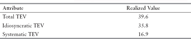
EXHIBIT 13.3 Position Amount of Individual Stocks in the Optimal Tracking Portfolio

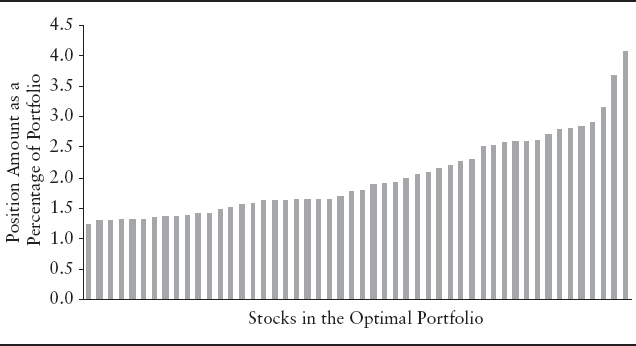
Exhibit 13.3 depicts the distribution of the position amount for individual stocks in the portfolio. We can see that the portfolio is well diversified across the 50 constituent stocks with no significant concentrations in any of the individual positions. The largest stock position is 4.1%, about three times larger than the smallest holding. Later in this chapter, we analyze the risk of this particular portfolio in more detail.

Constructing a Factor-Mimicking Portfolio

Factor-mimicking portfolios allow portfolio managers to capitalize on their views on various investment themes. For instance, the portfolio manager may forecast that small-cap stocks will outperform large-cap stocks or that value stocks will outperform growth stocks in the near future. By constructing long-short factor-mimicking portfolios, managers can place positions in line with their views on these investment themes without taking explicit directional views on the broader market.

Considering another example, suppose our portfolio manager forecasts that recent winner (high momentum) stocks will outperform recent losers (low momentum). To implement her views, she constructs two portfolios, one with winner stocks and one with loser stocks (100 stocks from the S&P 500 universe in each portfolio). She then takes a long position in the winners portfolio and a short position in the losers portfolio. While a sensible approach, a long-short portfolio constructed in this way would certainly have exposures to risk factors other than momentum. For instance, the momentum view might implicitly lead to unintended sector bets. If the portfolio manager wants to understand and potentially limit or avoid these exposures, she needs to perform further analysis. The use of a risk model will help her substantially.

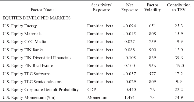
Exhibit 13.4 illustrates one of POINT^®'s risk model outputs—the 10 largest risk factor exposures by their contribution to TEV (last column in the exhibit) for this initial long-short portfolio. While momentum has the largest contribution to volatility, other risk factors also play a significant role. As a result, major moves in risk factors other than momentum can have a significant—and potentially unintended—impact on the portfolio's return.

EXHIBIT 13.4 Largest Risk Factor Exposures for the Momentum Winners/Losers Portfolio (bps/month)

Given this information, suppose our portfolio manager decides to avoid these exposures to the extent possible. She can do that by setting all exposures to factors other than momentum to zero (these type of constraints may not always be feasible and one may need to relax them to achieve a solution). Moreover, because she wants the portfolio to represent a pure systematic momentum effect, she seeks to minimize idiosyncratic risk. There are many ways to implement these goals, but increasingly portfolio managers are turning to risk models (using an optimization engine) to construct their portfolios in a robust and convenient way. She decides to setup an optimization problem where the objective function is the minimization of idiosyncratic risk. The tradable universe is the set of S&P 500 stocks and the portfolio is constructed to be dollar-neutral. This problem also incorporates the aforementioned factor exposure constraints.

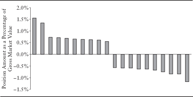
The resulting portfolio has exactly the risk factor exposures that were specified in the problem constraints. It exhibits a relatively low idiosyncratic TEV as a result of being well diversified with no significant concentrations in individual positions. Exhibit 13.5 depicts the largest 10 positions on the long and short sides of the momentum factor-mimicking portfolio; we see that there are no significant individual stock concentrations.

EXHIBIT 13.5 Largest 10 Positions on Long and Short Sides for the Momentum Portfolio

Implementing Sector Views

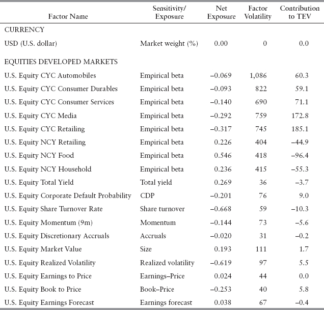
For our final portfolio construction example, let's assume we are entering a recessionary environment. An equity portfolio manager forecasts that the consumer staples sector will outperform the consumer discretionary sector in the near future, so she wants to create a portfolio to capitalize on this view. One simple idea would be to take a long position in the consumer staples sector (NCY: noncyclical) and a short position in the consumer discretionary sector (CYC: cyclical) by using, for example, sector ETFs. Similar to the previous example, this could result in exposures to risk factors other than the industry factors. Exhibit 13.6 illustrates the exposure of this long-short portfolio to the risk factors in the POINT^® U.S. equity risk model. As we can see in the table, the portfolio has significant net exposures to certain fundamental and technical factors, especially realized volatility and share turnover.

EXHIBIT 13.6 Factor Exposures and Contributions for Consumer Staples vs. Consumer Discretionary Portfolio (bps/month)

Suppose the portfolio manager decides to limit exposures to fundamental and technical factors. We can again use the optimizer to construct a long-short portfolio, with an exposure (beta) of 1 to the consumer staples sector and a beta of −1 to the consumer discretionary sector. To limit the exposure to fundamental and technical risk factors, we further impose the exposure to each of these factors to be between −0.2 and 0.2.⁹ We also restrict the portfolio to be dollar neutral, and allow for only long positions in the consumer staples stocks and for only short positions in consumer discretionary stocks. Finally, we restrict the investment universe to the members of the S&P 500 index¹⁰.

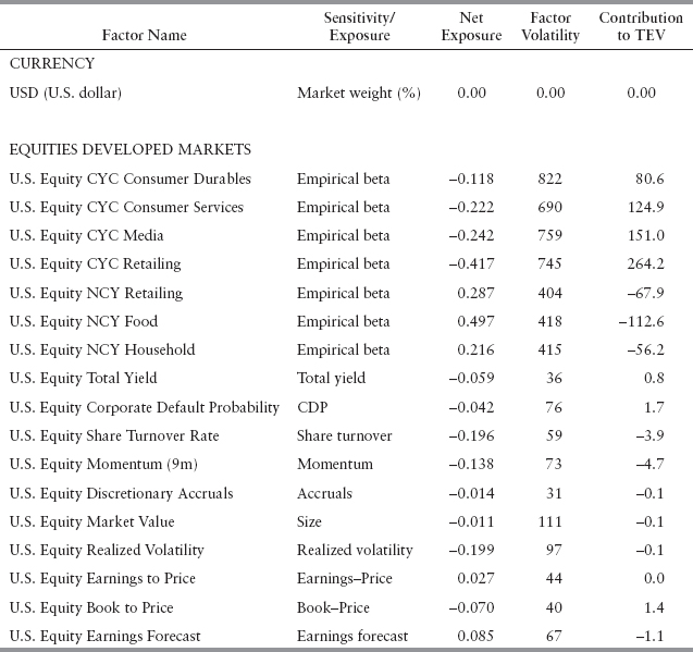
The resulting portfolio consists of 69 securities (approximately half of discretionary and staples stocks in S&P 500) with 31 long positions in the consumer staples stocks and 38 short positions in consumer discretionary stocks. Exhibit 13.7 depicts the factor exposures for this portfolio. As we can see in the table, the sum of the exposures to the industry factors is 1 for the consumer staples stocks and −1 for the consumer discretionary stocks. Exposures to fundamental and technical factors are generally significantly smaller when compared to the previous table, limiting the adverse effects of potential moves in these factors. Interestingly, no stocks from the automobiles industry are selected in the optimal portfolio, potentially due to excessive idiosyncratic risk of firms in that particular industry. The contribution to volatility from the discretionary sector is higher than that from the staples sector, due to higher volatility of industry factors in the discretionary sector.

The bounds used for the fundamental and technical factor exposures in the portfolio construction process were set to force a reduction in the exposure to these factors. However, there is a trade-off between having smaller exposures and having smaller idiosyncratic risk in the final portfolio. The resolution of this trade-off depends on the preferences of the portfolio manager. When the bounds are more restrictive, we are also decreasing the feasible set of solutions available to the problem and therefore potentially achieving a higher idiosyncratic risk (remember that the objective is the minimization of idiosyncratic risk). In our example, the idiosyncratic TEV of the portfolio increases from 119 bps/month (for staples—discretionary portfolio before the optimization) to 158 bps/month on the optimized portfolio. This change is the price paid for the ability to limit certain systematic risk factor exposures.

EXHIBIT 13.7 Factor Exposures and Contributions for the Optimal Sector View Portfolio (bps/month)

Analyzing Portfolio Risk Using Multifactor Models

Now that we have seen examples of using multifactor equity models for portfolio construction and briefly discussed their risk outcomes, we take a more in-depth look at portfolio risk. Risk analysis based on multifactor models can take many forms; from a relatively high-level aggregate approach, to an in-depth analysis of the risk properties of individual stocks and groups of stocks. Multifactor equity risk models provide the tools to perform the analysis of portfolio risk in many different dimensions, including exposures to risk factors, security factor contributions to total risk, analysis at the ticker level, and scenario analysis. In this section, we provide an overview of such detailed analysis using the S&P 500 index tracker example we created in the previous section.

Recall from Exhibit 13.2 that the TEV of the optimized S&P 500 tracking portfolio was 39.6 bps/month, composed mostly of idiosyncratic risk (35.8 bps/month) and a relatively small amount of systematic risk (16.9 bps/month). To analyze further the source of these numbers, we first compare the holdings of the portfolio with those of the benchmark and then study the impact of the mismatch to the risk of the net position (Portfolio – Benchmark). The first column in Exhibit 13.8 shows the net market weights (NMW) of the portfolio at the sector level (GICS level 1). Our portfolio appears to be well balanced with respect to the benchmark both from a market value and from a risk contribution perspective. The largest market value discrepancies are an overweight in information technology and an underweight in consumer discretionary and health care companies. However, the sector with the largest contribution to overall risk (contribution to TEV, or CTEV) is financials (7.5 bps/month). This may seem unexpected, given the small NMW of this sector (only 0.1%). This result is explained by the fact that contributions to risk (CTEV) are dependent on the net market weight, the risk of the underlying positions and also the correlation between the different exposures. Looking into the decomposition of the CTEV, the exhibit also shows that most of the total contribution to risk from financials is idiosyncratic (7.0 bps/month). This result is due to the small number of securities our portfolio has in this sector and the underlying high volatility of these stocks. In short, the diversification benefits across financial stocks are small in our portfolio: we could potentially significantly reduce total risk by constructing our financials exposure using more names. Note that this analysis is only possible with a risk model.

EXHIBIT 13.8 Net Market Weights and Risk Contributions by Sector (bps/month)

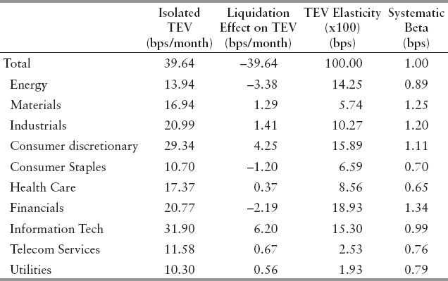
Exhibit 13.9 highlights additional risk measures by sector. What we see in the first column is the isolated TEV, that is, the risk associated with the stocks in that particular sector only. On an isolated basis, the information technology sector has the highest risk in the portfolio. This top position in terms of isolated risk does not translate into the highest contribution to overall portfolio risk, as we saw in Exhibit 13.8. The discrepancy between isolated risk numbers and contributions to risk is explained by the correlation between the exposures and allows us to understand the potential hedging effects present across our portfolio. The liquidation effect reported in the table represents the change in TEV when we completely hedge that particular position, that is, enforce zero net exposure to any stock in that particular sector. Interestingly, eliminating our exposure to information technology stocks would actually increase our overall portfolio risk by 6.2 bps/month. This happens because the overweight in this sector is effectively hedging out risk contributions from other sectors. If we eliminate this exposure, the portfolio balance is compromised. The TEV elasticity reported gives an additional perspective regarding how the TEV in the portfolio changes when we change the exposure to that sector. Specifically, it tells us the percentage change in TEV for each 1% change in our exposure to that particular sector. For example, if we double our exposure to the energy sector, our TEV would increase by 14.25% (from 39.6 bps/month to 45.2 bps/month). Finally, the report estimates the portfolio to have a beta of 1.00 to the benchmark, which is, of course, in line with our index tracking objective. The beta statistic measures the comovement between the systematic risk drivers of the portfolio and the benchmark and should be interpreted only as that. In particular, a low portfolio beta (relative to the benchmark) does not imply low portfolio risk. It signals relatively low systematic co-movement between the two universes or a relatively high idiosyncratic risk for the portfolio. For example, if the sources of systematic risk from the portfolio and the benchmark are distinct, the portfolio beta is close to zero. The report also provides the systematic beta associated with each sector. For instance, we see that a movement of 1% in the benchmark leads to a 1.34% return in the financials component of our portfolio. As expected, consumer staples and health care are two low beta industries, as they tend to be more stable through the business cycle.¹¹

EXHIBIT 13.9 Additional Risk Measures by Sector

Although important, the information we examined so far is still quite aggregated. For instance, we know from Exhibit 13.8 that a large component of idiosyncratic risk comes from financials. But what names are contributing most? What are the most volatile sectors? How are systematic exposures distributed within each sector? Risk models should be able to provide answers to all these questions, allowing for a detailed view of the portfolio's risk exposures and contributions. As an example, Exhibit 13.10 displays all systematic risk factors the portfolio or the benchmark loads onto. It also provides the portfolio, benchmark, and net exposures for each risk factor, the volatility of each of these factors, and their contributions to total TEV. The table shows that the net exposures to the risk factors are generally low, meaning that the tracking portfolio has small active exposures. This finding is in line with the evidence from Exhibit 13.2, where we see that the systematic risk is small (16.9 bps/month). If we look into the contributions of individual factors to total TEV, the exhibit shows that the top contributors are the size, share turnover, and realized volatility factors. The optimal index tracking portfolio tends to be composed of very large-cap names within the specified universe, and that explains the net positive loading to the market value (size) factor. This portfolio tilt is due to the generally low idiosyncratic risk large companies have. This is seen favorably by the optimization engine, as it tries to minimize idiosyncratic risk. This same tilt would explain our net exposure to both the share turnover and realized volatility factors, as larger companies tend to have lower realized volatility and share turnover too. Interestingly, industry factors have relatively small contributions to TEV, even though they exhibit significantly higher volatilities. This results from the fact that the optimization engine specifically targets these factors because of their high volatility and is successful in minimizing net exposure to industry factors in the final portfolio.

EXHIBIT 13.10 Factor Exposures and Contributions for the Tracking Portfolio vs. S&P 500 (bps/month)

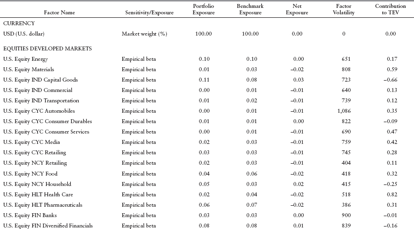
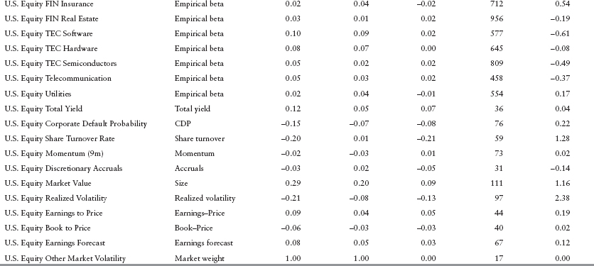
EXHIBIT 13.11 Individual Securities and Idiosyncratic Risk Exposures

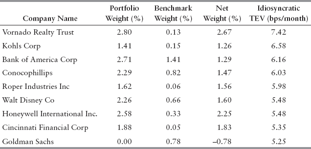
Finally, remember from Exhibit 13.2 that the largest component of the portfolio risk comes from name-specific exposures. Therefore, it is important to be aware of which individual stocks in our portfolio contribute the most to overall risk. Exhibit 13.11 shows the set of stocks in our portfolio with the largest idiosyncratic risk. The portfolio manager can use this information as a screening device to filter out undesirable positions with high idiosyncratic risk and to make sure her views on individual firms translate into risk as expected. In particular, the list in the exhibit should only include names about which the portfolio manager has strong views, either positive—expressed with positive NMW—or negative—in which case we would expect a short net position.

It should be clear from the above examples that although the factors used to measure risk are predetermined in a linear factor model, there is a large amount of flexibility on the way the risk numbers can be aggregated and reported. Instead of sectors, we could have grouped risk by any other classification of individual stocks, for example, by regions or market capitalization. This allows the risk to be reported using the same investment philosophy underlying the portfolio construction process¹² regardless of the underlying factor model. There are also many other risk analytics available not mentioned in this example that give additional detail about specific risk properties of the portfolio and the constituents. We have only discussed total, systematic, and idiosyncratic risk (which can be decomposed into risk contributions on a flexible basis), and referred to isolated and liquidation TEV, TEV elasticity, and portfolio beta. Most users of multifactor risk models will find their own preferred approach to risk analysis through experience.

Performance Attribution

Now that we discussed portfolio construction and risk analysis as the first steps of the investment process, we give a brief overview of performance attribution, an ex post analysis of performance typically conducted at the end of the investment horizon. Performance attribution analysis provides an evaluation of the portfolio manager's performance with respect to various decisions made throughout the investment process. The underperformance or outperformance of the portfolio manager, when compared to the benchmark can be due to different reasons including effective sector allocation, security selection, or tilting the portfolio towards certain risk factors. Attribution analysis aims to unravel the major sources of this performance differential. The exercise allows the portfolio manager to understand how her particular views—translated into net exposures—performed during the period and reveals whether some of the portfolio's performance was the result of unintended bets.

There are three basic forms of attribution analysis used for equity portfolios. These are return decomposition, factor model–based attribution, and style analysis. In the return decomposition approach, the performance of the portfolio manager is generally attributed to top-down allocation (e.g., currency, country, or sector allocation) in a first step, followed by a bottom-up security selection performance analysis. This is a widely used technique among equity portfolio managers.

Factor model–based analysis attributes performance to exposures to risk factors such as industry, size, and financial ratios. It is relatively more complicated than the previous approach and is based on a particular risk model that needs to be well understood. For example, let's assume that a portfolio manager forecasts that value stocks will outperform growth stocks in the near future. As a result, the manager tilts the portfolio toward value stocks as compared to the benchmark, creating an active exposure to the value factor. In an attribution framework without systematic factors, such sources of performance cannot be identified and hence may be inadvertently attributed to other reasons. Factor model–based attribution analysis adds value by incorporating these factors (representing major investment themes) explicitly into the return decomposition process and by identifying additional sources of performance represented as active exposures to systematic risk factors.

Style analysis on the other hand is based on a regression of the portfolio return to a set of style benchmarks. It requires very little information (e.g., we do not need to know the contents of the portfolio) but the outcome depends significantly on the selection of style benchmarks. It also assumes constant loadings to these styles across the regression period, which may be unrealistic for managers with somewhat dynamic allocations.

Factor–Based Scenario Analysis

The last application we review in this chapter goes over the use of equity risk factor models in the context of scenario analysis. Many investment professionals utilize scenario analysis in different shapes and forms for both risk and portfolio construction purposes. Factor-based scenario analysis is a tool that helps portfolio managers in their decision making process by providing additional intuition on the behavior of their portfolio under a specified scenario. A scenario can be a historical episode, such as the equity market crash of 1987, the war in Iraq, or the 2008 credit crisis. Alternatively, scenarios can be defined as a collection of hypothetical views (e.g., user-defined scenarios) in a variety of forms such as a view on a given portfolio or index (e.g., S&P 500 drops by 20%) or a factor (e.g., U.S. equity–size factor moves by 3 standard deviations) or correlation between factors (e.g., increasing correlations across markets in episodes of flight to quality). In this section, we use the POINT^® Factor-Based Scenario Analysis Tool to illustrate how we can utilize factor models to perform scenario analysis.

Before we start describing the example, let's take an overview of the mechanics of the model. It allows for the specification of user views on returns of portfolios, indexes, or risk factors. When the user specifies a view on a portfolio or index, this is translated into a view on risk factor realizations, through the linear factor model framework.¹³ These views are combined with ones that are directly specified in terms of risk factors. It is important to note that the portfolio manager does not need to specify views on all risk factors, and typically has views only on a small subset of them. Once the manager specifies this subset of original views, the next step is to expand these views to the whole set of factors. The scenario analysis engine achieves this by estimating the most likely realization of all other factors—given the factor realizations on which views are specified—using the risk model covariance matrix. Once all factors realizations are populated, the scenario outcome for any portfolio or index can be computed by multiplying their specific exposures to the risk factors by the factor realizations under the scenario. The tool provides a detailed analysis of the portfolio behavior under the specified scenario.

EXHIBIT 13.12 Index Returns under Scenario 1 (VIX jumps by 50%)

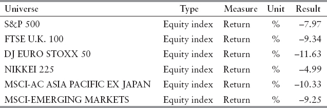
We illustrate this tool using two different scenarios: a 50% shift in the U.S. equity market volatility—represented by the VIX index—(scenario 1) and a 50% jump in the European credit spreads (scenario 2).¹⁴ We use a set of equity indexes from across the globe to illustrate the impact of these two scenarios. We run the scenarios as of July 30, 2010, which specifies the date both for the index loadings and the covariance matrix used. Base currency is set to U.S. dollars (USD) and hence index returns presented below are in USD.

Exhibit 13.12 shows the returns of the chosen equity indexes under the first scenario. We see that all indexes experience significant negative returns with Euro Stoxx plummeting the most and Nikkei experiencing the smallest drop. To understand these numbers better, let's look into the contributions of different factors to these index returns.

Exhibit 13.13 illustrates return contributions for four of these equity indexes under scenario 1. Specifically, for each index, it decomposes the total scenario return into return coming from different factors each index has exposure to. In this example, all currency factors are defined with respect to USD. Moreover, equity factors are expressed in their corresponding local currencies and can be described as broad market factors for their respective regions.

Not surprisingly, Exhibit 13.13 shows that the majority of the return contributions for selected indexes come from the reaction of equity market factors to the scenario. However, foreign exchange (FX) can also be a significant portion of total return for some indexes, such as in the case of the Euro Stoxx (−4.8%). Nikkei experiences a relatively smaller drop in USD terms, majorly due to a positive contribution coming from the JPY FX factor. This positive contribution is due to the safe haven nature of Japanese yen in case of flight to quality under increased risk aversion in global markets.

EXHIBIT 13.13 Return Contributions for Equity Indexes under Scenario 1 (in %)

EXHIBIT 13.14 Factor Returns and Z-Scores under Scenario 1

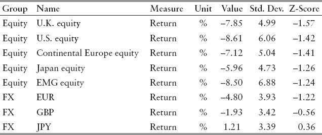
Exhibit 13.14 demonstrates the scenario implied factor realizations (value), factor volatilities, and the Z-scores for the risk factors given in Exhibit 13.13. The Z-score of the factor quantifies the effect of the scenario on that specific factor. It is computed as

where r is the return of the factor in the scenario and σ_r is the standard deviation of the factor. Hence, the Z-score measures how many standard deviations a factor moves in a given scenario. Exhibit 13.14 lists the factors by increasing Z-score under scenario 1. The U.K. equity factor experiences the largest negative move, at −1.57 standard deviations. FX factors experience relatively smaller movements. JPY is the only factor with a positive realization due to the aforementioned characteristic of the currency.

EXHIBIT 13.15 Index Returns under Scenario 2 (EUR Credit Spread Jumps by 50%)

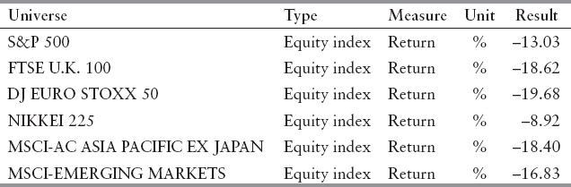
EXHIBIT 13.16 Factor Returns and Z-Scores under Scenario 2

In the second scenario, we shift European credit spreads by 50% (a 3.5-sigma event) and explore the effect of credit market swings on the equity markets. As we can see in Exhibit 13.15, all equity indexes experience significant returns, in line with the severity of the scenario.¹⁵ The result also underpins the strong recent co-movement between the credit and equity markets. The exception is again the Nikkei that realizes a relatively smaller return.

Exhibit 13.16 provides the return, volatility, and the Z-score of certain relevant factors under scenario 2. As expected, the major mover on the equity side is the continental Europe equity factor, followed by the United Kingdom. Given the recent strong correlations between equity and credit markets across the globe, the exhibit suggests that a 3.5 standard deviation shift in the European spread factor results in 2 to 3 standard deviation movement of global equity factors.

The two examples above illustrate the use of factor models in performing scenario analysis to achieve a clear understanding of how a portfolio may react under different circumstances.