ANALYSIS OF FACTOR DATA

After constructing factors for all securities in the investable universe, each factor is analyzed individually. Presenting the time-series and cross-sectional averages of the mean, standard deviations, and key percentiles of the distribution provide useful information for understanding the behavior of the chosen factors.

Although we often rely on techniques that assume the underlying data generating process is normally distributed, or at least approximately, most financial data is not. The underlying data generating processes that embody aggregate investor behavior and characterize the financial markets are unknown and exhibit significant uncertainty. Investor behavior is uncertain because not all investors make rational decisions or have the same goals. Analyzing the properties of data may help us better understand how uncertainty affects our choice and calibration of a model.

Below we provide some examples of the cross-sectional characteristics of various factors. For ease of exposition we use histograms to evaluate the data rather than formal statistical tests. We let particular patterns or properties of the histograms guide us in the choice of the appropriate technique to model the factor. We recommend that an intuitive exploration should be followed by a more formal statistical testing procedure. Our approach here is to analyze the entire sample, all positive values, all negative values, and zero values. Although omitted here, a thorough analysis should also include separate subsample analysis.

Example 1: EBITDA/EV

The first factor we discuss is the earnings before interest taxes and amortization to enterprise value (EBITDA/EV) factor. Enterprise value is calculated as the market value of the capital structure. This factor measures the price (enterprise value) investors pays to receive the cash flows (EBITDA) of a company. The economic intuition underlying this factor is that the valuation of a company's cash flow determines the attractiveness of companies to an investor.

Exhibit 11.3(A) presents a histogram of all cross-sectional values of the EBITDA/EV factor throughout the entire history of the study. The distribution is close to normal, showing there is a fairly symmetric dispersion among the valuations companies receive. Exhibit 11.3(B) shows that the distribution of all the positive values of the factor is also almost normally distributed. On the other hand, Exhibit 11.3(C) shows that the distribution of the negative values is skewed to the left. However, because there are only a small number of negative values, it is likely that they will not greatly influence our model.

Example 2: Revisions

We evaluate the cross-sectional distribution of the earnings revisions factor.¹⁸ The revisions factor we use is derived from sell-side analyst earnings forecasts from the IBES database. The factor is calculated as the number of analysts who revise their earnings forecast upward minus the number of downward forecasts, divided by the total number of forecasts. The economic intuition underlying this factor is that there should be a positive relation to changes in forecasts of earnings and subsequent returns.

In Exhibit 11.4(A) we see that the distribution of revisions is symmetric and leptokurtic around a mean of about zero. This distribution ties with the economic intuition behind the revisions. Since business prospects of companies typically do not change from month-to-month, sell-side analysts will not revise their earnings forecast every month. Consequently, we expect and find the cross-sectional range to be peaked at zero. Exhibit 11.4(B) and (C), respectively, show there is a smaller number of both positive and negative earnings revisions and each one of these distributions are skewed.

Example 3: Share Repurchase

We evaluate the cross-sectional distribution of the shares repurchases factor. This factor is calculated as the difference of the current number of common shares outstanding and the number of shares outstanding 12 months ago, divided by the number of shares outstanding 12 months ago. The economic intuition underlying this factor is that share repurchase provides information to investors about future earnings and valuation of the company's stock.¹⁹ We expect there to be a positive relationship between a reduction in shares outstanding and subsequent returns.

EXHIBIT 11.3 Histograms of the Cross-Sectional Values for the EBITDA/EV Factor A. All Factor Values

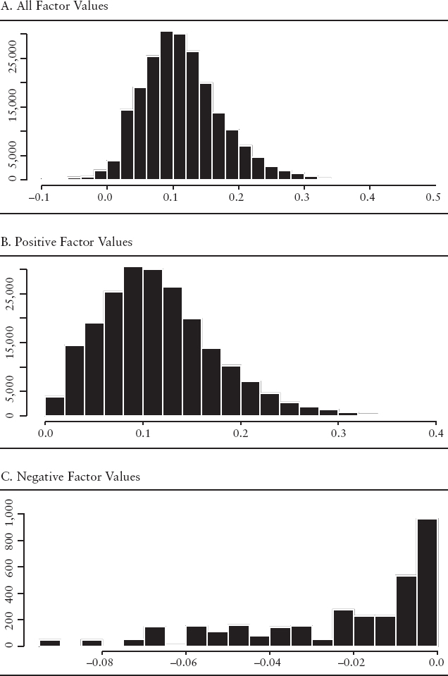
EXHIBIT 11.4 Histograms of the Cross-Sectional Values for the Revisions Factor A. All Factor Values

We see in Exhibit 11.5(A) that the distribution is leptokurtic. The positive values (see Exhibit 11.5(B)) are skewed to the right and the negative values (see Exhibit 11.5(C)) are clustered in a small band. The economic intuition underlying share repurchases is the following. Firms with increasing share count indicate they require additional sources of cash. This need could be an early sign that the firm is experiencing higher operating risks or financial distress. We would expect these firms to have lower future returns. Firms with decreasing share count have excess cash and are returning value back to shareholders. Decreasing share count could result because management believes the shares are undervalued. As expected, we find the cross-sectional range to be peaked at zero (see Exhibit 11.5(D)) since not all firms issue or repurchase shares on a regular basis.