
DISENTANGLING
The effects of different sources of stock return can overlap. In Exhibit 7.1, the lines represent connections documented by academic studies; they may appear like a ball of yarn after the cat got to it. To unravel the connections between predictor variables and return, it is necessary to examine all the variables simultaneously.
For instance, the low P/E effect is widely recognized, as is the small-size effect. But stocks with low P/Es also tend to be of small size. Are P/E and size merely two ways of looking at the same effect? Or does each variable matter? Perhaps the excess returns to small-cap stocks are merely a January effect, reflecting the tendency of taxable investors to sell depressed stocks at year-end. Answering these questions requires disentangling return effects via multivariate regression.5
Common methods of measuring return effects (such as quintiling or univariate, single-variable, regression) are naive because they assume, naively, that prices are responding only to the single variable under consideration, low P/E, say. But a number of related variables may be affecting returns. As we have noted, small-cap stocks and banking and utility industry stocks tend to have low P/Es. A univariate regression of return on low P/E will capture, along with the effect of P/E, a great deal of noise related to firm size, industry affiliation, and other variables.
EXHIBIT 7.1 Return Effects Form a Tangled Web

Simultaneous analysis of all relevant variables via multivariate regression takes into account and adjusts for such interrelationships. The result is the return to each variable separately, controlling for all related variables. A multivariate analysis for low P/E, for example, will provide a measure of the excess return to a portfolio that is market-like in all respects except for having a lower-than-average P/E ratio. Disentangled returns are pure returns.
Noise Reduction
Exhibit 7.2 plots naive and pure cumulative monthly excess (relative to a 3,000-stock universe) returns to high book–price ratio (B/P). (Conceptually, naive and pure returns come from a portfolio having a B/P that is one standard deviation above the universe mean B/P; for the pure returns, the portfolio is also constrained to have universe-average exposures to all the other variables in the model, including fundamental characteristics and industry affiliations.) The naive returns show a great deal of volatility; the pure returns, by contrast, follow a much smoother path. There is a lot of noise in the naive returns. What causes it?
EXHIBIT 7.2 Naive and Pure Returns to High Book-to-Price Ratio

Notice the divergence between the naive and pure return series for the 12 months starting in March 1979. This date coincides with the crisis at Three Mile Island nuclear power plant. Utilities such as GPU, operator of the Three Mile Island power plant, tend to have high B/Ps, and naive B/P measures will reflect the performance of these utilities along with the performance of other high-B/P stocks. Electric utility prices plummeted 24% after the Three Mile Island crisis. The naive B/P measure reflects this decline.
But industry-related events such as Three Mile Island have no necessary bearing on the B/P variable. An investor could, for example, hold a high-B/P portfolio that does not overweight utilities, and such a portfolio would not have experienced the decline reflected in the naive B/P measure in Exhibit 7.2. The naive returns to B/P reflect noise from the inclusion of a utility industry effect. A pure B/P measure is not contaminated by such irrelevant variables.
Disentangling distinguishes real effects from mere proxies and thereby distinguishes between real and spurious investment opportunities. As it separates high B/P and industry affiliation, for example, it can also separate the effects of firm size from the effects of related variables. Disentangling shows that returns to small firms in January are not abnormal; the apparent January seasonal merely proxies for year-end tax-loss selling.6 Not all small firms will benefit from a January rebound; indiscriminately buying small firms at the turn of the year is not an optimal investment strategy. Ascertaining true causation leads to more profitable strategies.
Return Revelation
Disentangling can reveal hidden opportunities. Exhibit 7.3 plots the naively measured cumulative monthly excess returns (relative to the 3,000-stock universe) to portfolios that rank lower than average in market capitalization and price per share and higher than average in terms of analyst neglect. These results derive from monthly univariate regressions. The small-cap line thus represents the cumulative excess returns to a portfolio of stocks naively chosen on the basis of their size, with no attempt made to control for other variables.
All three return series move together. The similarity between the small-cap and neglect series is particularly striking. This is confirmed by the correlation coefficients in the first column of Exhibit 7.4. Furthermore, all series show a great deal of volatility within a broader up, down, up pattern.
EXHIBIT 7.3 Naive Returns Can Hide Opportunities: Three Size-Related Variables
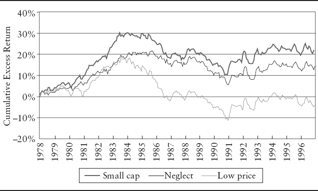
EXHIBIT 7.4 Correlations Between Monthly Returns to Size-Related Variablesa

EXHIBIT 7.5 Pure Returns Can Reveal Opportunities: Three Size-Related Variables
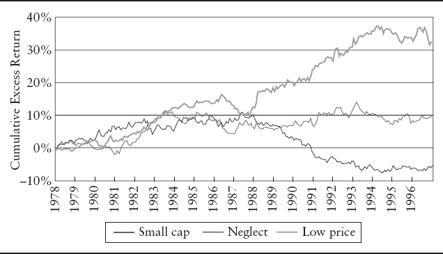
Exhibit 7.5 shows the pure cumulative monthly excess returns to each size-related attribute over the period. These disentangled returns adjust for correlations not only between the three size variables, but also between each size variable and industry affiliations and each variable and growth and value characteristics. Two findings are immediately apparent from Exhibit 7.5.
First, pure returns to the size variables do not appear to be nearly as closely correlated as the naive returns displayed in Exhibit 7.3. In fact, over the second half of the period, the three return series diverge substantially. This is confirmed by the correlation coefficients in the second column of Exhibit 7.4.
In particular, pure returns to small capitalization accumulate quite a gain over the period; they are up 30%, versus an only 20% gain for the naive returns to small cap. Purifying returns reveals a profit opportunity not apparent in the naive returns. Furthermore, pure returns to analyst neglect amount to a substantial loss over the period. Because disentangling controls for proxy effects, and thereby avoids redundancies, these pure return effects are additive. A portfolio could have aimed for superior returns by selecting small-cap stocks with a higher-than-average analyst following (that is, a negative exposure to analyst neglect).
EXHIBIT 7.6 Pure Returns Are Less Volatile, More Predictable: Standard Deviations of Monthly Returns to Size-Related Variablesa

Second, the pure returns appear to be much less volatile than the naive returns. The naive returns in Exhibit 7.3 display much month-to-month volatility within their more general trends. By contrast, the pure series in Exhibit 7.5 are much smoother and more consistent. This is confirmed by the standard deviations given in Exhibit 7.6.
The pure returns in Exhibit 7.5 are smoother and more consistent than the naive return responses in Exhibit 7.3 because the pure returns capture more signal and less noise. And because they are smoother and more consistent than naive returns, pure returns are also more predictive.
Predictive Power
Disentangling improves the predictive power of estimated returns by providing a clearer picture of the relationships between investor behavior, fundamental variables, and macroeconomic conditions. For example, investors often prefer value stocks in bearish market environments, because growth stocks are priced more on the basis of high expectations, which get dashed in more pessimistic eras. But the success of such a strategy will depend on the variables one has chosen to define value.
Exhibit 7.7 displays the results of regressing both naive and pure monthly returns to various value-related variables on market (S&P 500) returns over the 1978–1996 period. The results indicate that DDM value is a poor indicator of a stock's ability to withstand a tide of receding market prices. The regression coefficient in the first column indicates that a portfolio with a one-standard-deviation exposure to DDM value will tend to outperform by 0.06% when the market rises by 1.00% and to underperform by a similar margin when the market falls by 1.00%. The coefficient for pure returns to DDM is similar. Whether their returns are measured in pure or naive form, stocks with high DDM values tend to behave procyclically.
EXHIBIT 7.7 Market Sensitivities of Monthly Returns to Value-Related Variables
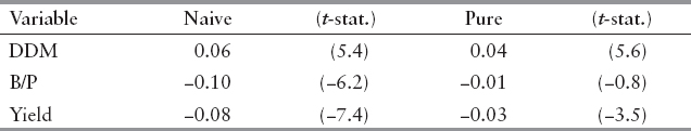
High B/P appears to be a better indicator of a defensive stock. It has a regression coefficient of –0.10 in naive form. In pure form, however, B/P is virtually uncorrelated with market movements; pure B/P signals neither an aggressive nor a defensive stock. B/P as naively measured apparently picks up the effects of truly defensive variables, such as high yield.
The value investor in search of a defensive posture in uncertain market climates should consider moving toward high yield. The regression coefficients for both naive and pure returns to high yield indicate significant negative market sensitivities. Stocks with high yields may be expected to lag in up markets but to hold up relatively well during general market declines.
These results make broad intuitive sense. DDM is forward-looking, relying on estimates of future earnings. In bull markets, investors take a long-term outlook, so DDM explains security pricing behavior. In bear markets, however, investors become myopic; they prefer today's tangible income to tomorrow's promise. Current yield is rewarded.
Pure returns respond in intuitively satisfying ways to macroeconomic events. Exhibit 7.8 illustrates, as an example, the estimated effects of changes in various macroeconomic variables on the pure returns to small size (as measured by market capitalization). Consistent with the capital constraints on small firms and their relatively greater sensitivity to the economy, pure returns to small size may be expected to be negative in the first four months following an unexpected increase in the Baa corporate rate and positive in the first month following an unexpected increase in industrial production.7 Investors can exploit such predictable behavior by moving into and out of the small-cap market segment as economic conditions evolve.8
These examples serve to illustrate that the use of numerous, finely defined fundamental variables can provide a rich representation of the complexity of security pricing. The model can be even more finely tuned, however, by including variables that capture such subtleties as the effects of investor psychology, possible nonlinearities in variable-return relationships, and security transaction costs.
EXHIBIT 7.8 Forecast Response of Small Size to Macroeconomic Shocks

Additional Complexities
In considering possible variables for inclusion in a model of stock price behavior, the investor should recognize that pure stock returns are driven by a combination of economic fundamentals and investor psychology. That is, economic fundamentals such as interest rates, industrial production, and inflation can explain much, but by no means all, of the systematic variation in returns. Psychology, including investors' tendency to overreact, their desire to seek safety in numbers, and their selective memories, also plays a role in security pricing.
What's more, the modeler should realize that the effects of different variables, fundamental and otherwise, can differ across different types of stocks. The value sector, for example, includes more financial stocks than the growth sector. Investors may thus expect value stocks in general to be more sensitive than growth stocks to changes in interest rate spreads.
Psychologically based variables such as short-term overreaction and price correction also seem to have a stronger effect on value than on growth stocks. Earnings surprises and earnings estimate revisions, by contrast, appear to be more important for growth than for value stocks. Thus, Google shares can take a nosedive when earnings come in a penny under expectations, whereas Duke Energy shares remain unmoved even by fairly substantial departures of actual earnings from expectations.
The relationship between stock returns and relevant variables may not be linear. The effects of positive earnings surprises, for instance, tend to be arbitraged away quickly; thus positive earnings surprises offer less opportunity for the investor. The effects of negative earnings surprises, however, appear to be more long-lasting. This nonlinearity may reflect the fact that sales of stock are limited to those investors who already own the stock (and to a relatively small number of short sellers).9
Risk-variable relationships may also differ across different types of stock. In particular, small-cap stocks generally have more idiosyncratic risk than large-cap stocks. Diversification is thus more important for small-stock than for large-stock portfolios.
Return-variable relationships can also change over time. Recall the difference between DDM and yield value measures: high-DDM stocks tend to have high returns in bull markets and low returns in bear markets; high-yield stocks experience the reverse. For consistency of performance, return modeling must consider the effects of market dynamics, the changing nature of the overall market.
The investor may also want to decipher the informational signals generated by informed agents. Corporate decisions to issue or buy back shares, split stock, or initiate or suspend dividends, for example, may contain valuable information about company prospects. So, too, may insiders' (legal) trading in their own firms' shares.
Finally, a complex model containing multiple variables is likely to turn up a number of promising return-variable relationships. But are these perceived profit opportunities translatable into real economic opportunities? Are some too ephemeral? Too small to survive frictions such as trading costs? Estimates of expected returns must be combined with estimates of the costs of trading to arrive at realistic returns net of trading costs.