
P/E MYOPIA: THE FALLACY OF A STABLE P/E
To this point, we have utilized projections of future investments and returns to calculate the theoretical prospective P/E ratio at a single point in time. We now take a multiyear look at the time evolution of the relationship between realized earnings growth and realized P/E.
When estimating future earnings growth, historical earnings growth is the commonly used baseline around which an analyst will make some (typically modest) adjustments. Price appreciation is often assumed to follow the projected earnings growth with P/E remaining stable. In this way, investors tacitly elevate earnings growth to the central determinant of investment value.
Theoretically, stable P/Es are unlikely to be achieved, even under equilibrium conditions in which market returns and a company's long-term prospects remain stable. Rather there is a natural time-path of P/E evolution. This observation stands in stark contrast to the valuation methodology typically used to estimate the long-term potential of investment banking deals involving mergers, acquisitions and buyouts. In such valuations, growing earnings are projected along with a horizon P/E that is close to the current value. The combination of these growth and stability assumptions is likely to lead to excessively optimistic estimates of the IRR (internal rate of return) potential of such deals.
Given current P/E values, we ask how the P/E theoretically changes over subsequent years under varying earnings growth assumptions. By analogy to fixed income terminology, we label the equilibrium-implied future P/E, the P/E forward. We call the trace over time the P/E orbit. This seemingly straightforward approach leads to a number of striking implications. For example, it shows that high growth stocks can induce a P/E myopia, leading otherwise thoughtful analysts to an overestimation of holding-period returns.
In order to fruitfully discuss P/E orbits, we need to review a few basic relationships. The first of these relationships is the basic single-period return produced by an equity investment. The holding-period return is the sum of just two quantities, the dividend yield (DY), and price return (% price change):
![]()
The dividend yield is usually fairly stable, so this component of return will provide a reliable, steady addition to return. Price return is more variable and is therefore the critical ingredient in return volatility. The price return can be shown mathematically to be the sum of the growth in earnings, gE, and growth in P/E, gP/E, over the holding period:
![]()
Armed with these basic formulas, we can compare the P/E orbit of a high growth stock with the P/E orbit of a low growth stock. We will use a numerical example, starting with k = 9% as the market discount rate for all stocks discussed in this chapter. In reality, of course, the discount rate varies from company to company, with changing market conditions, and should probably even be used to differentiate the risk prospects of the TV from the FV. If our hypothetical stock is fairly priced, it will provide a 9% holding period return. This equilibrium return assumption tells us a great deal about what theoretically should be happening to the P/E.
The discount rate k will actually change over time along with changes in interest rates and equity risk premiums. However, for simplicity and clarity we discount all earnings at a fixed k = 9%.
P/E Orbits for High-Growth Stocks
Suppose the stock of the high-growth Firm D trades at a P/E multiple of 25×. The expected earnings growth is 12.4% (the rationale for choosing this particular growth rate will become evident later) and the dividend yield is 1.6%.
Since the holding period return is the sum of the dividend yield and the price return, a 9% return and a 1.6% dividend yield implies that the price return must be 7.4% (9% – 1.6%). Repeating the formula above:

This result suggests that, over a one-year holding period, the P/E is implicitly expected to fall –5% from the current 25× to a forward P/E of 23.8×.
At first, this result is surprising. Why should the P/E register such a sharp decline over the course of a single year, especially after a 12.4% growth in earnings? The result is a direct consequence of our assumption that the initial P/E of 25× represents fair equilibrium pricing. The fair pricing assumption implies that, given the long-term prospects for the company, an appropriately specified valuation model would validate the P/E of 25× if the earnings discount rate was 9%. In this example, the first year of earnings growth was specified at 12.4%.
The P/E decline is also implicitly related to the assumption that, at the outset, the firm has a fixed FV that is consumed/utilized over time. High earnings growth in the early years can then be viewed as leading to rapid realization of the firm's potential.
We note that earnings growth rates can fluctuate widely from year-to-year and long-term growth forecasts are shrouded in more uncertainty short-term forecasts. In actuality, many future sequences of subsequent annual earnings growth rates can lead to the precisely the same initial fair value P/E of 25×.
Regardless of the future earnings growth path, an equilibrium 9% return assumption and 12.4% first year growth necessitates an expected 5% P/E decline and a new year-end fair value of 23.8×.
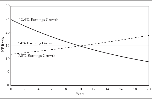
As long as Firm D's earnings growth rate remains at 12.4% and the market discount rate stays at 9%, the P/E should continue to decline by 5%. Thus, in the second year the P/E should decline from 23.8× to 22.6×. Continuing at this rate for 10 years brings the P/E down to 15×, as depicted in the curve that emanates from a P/E of 25× in Exhibit 3.6.
As an example, imagine a pharmaceutical company currently enjoying a healthy 12.4% earnings growth from sales of a proprietary drug. If the drug goes generic and the company's research pipeline is unpromising, the eroding franchise (i.e., the consumption of FV) will be reflected in a corresponding decline in P/E.
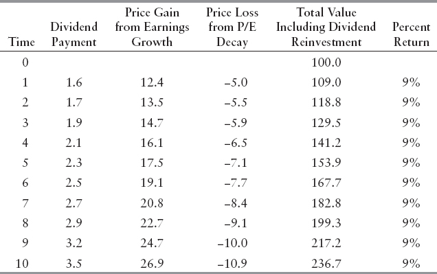
A few words of caution are needed so that Exhibit 3.6 is not misinterpreted. First, the descending P/E orbit does not imply a decline in the equity price. The 12.4% earnings growth brings investment gains that more than offset losses due to the P/E induced 5% price decline. The corresponding stock price trajectory will be one of 7.4% positive growth. When we add a 1.6% dividend to 7.4% price growth we achieve a 9% return, just as we would expect with a 9% discount rate. Exhibit 3.7 illustrates how dividends, earnings growth and P/E decay combine to provide a 9% annual return.
EXHIBIT 3.6 P/E Orbits with Constant Earnings Growth
The basic assumption is that the initial P/E of 25× represents fair-value discounting of the company's future earnings growth. But, the high 12.4% level of earnings growth cannot continue indefinitely. With a 9% discount rate, perpetual earnings growth at 12.4% would require an infinite starting P/E and necessarily violates the assumption that 25× represents fair pricing. The 12.4% curve in Exhibit 3.6 should be viewed as portraying the P/E descent for just so long as earnings growth remains at 12.4%.
The depicted P/E orbit does not depend on the choice of 25× as the starting P/E. As long as k = 9% and g = 12.4%, the projected P/E “should” decline by 5% each and every year. Under these return and growth and assumptions, the same 5% year over year decline will apply for all initial P/E values!
There may be a myriad of reasons why a specific investor may hold to the belief that the P/E will not experience any such decline—improvement in the stock's prospects, the market's better appreciation of the stock's promise, the salutary effect of realized earnings growth (even if it only confirms the previously expected high 12.4% level), general market improvements, changes in required discount rates, and so on. All of these events constitute a departure, however, from the equilibrium conditions as they have been defined. Hence, excluding the P/E movements induced by such nonequilibrium factors that result in unanticipated additions to FV, the stock's P/E should decline by 5%.
EXHIBIT 3.7 Growth of $100 Investment (1.6% dividend, 12.4% earnings growth, -5%. P/E decline
P/E Orbits for Low-Growth Stocks
For low-growth stocks, the same formulation as above also leads to continuous P/E change, but the change results in an ascending P/E orbit, as displayed in the 5% growth curve in Exhibit 3.6. If the starting P/E is 11.8× and the same 1.6% dividend yield and 9% market discount rate as in the previous example apply, the P/E will grow to 15× over 10 years.
Moving toward a higher P/E in the face of lower earnings growth seems contrary to basic intuition but it does make sense when we think in terms of FV consumption. High-growth firms rapidly consume their FV while low-growth firms consume FV slowly. In the equilibrium framework, the consensus investor expects a 9% total return. With a 1.6% dividend yield and expected 5% earnings growth, the only way we can reach that return is through expected P/E growth of 2.4%! Any P/E growth below this “required level” will be disappointing, and any greater increase will be a source of excess return.
The P/E orbit for g = 5% appears to rise without limit. Of course, this cannot be, either in practice or in any reasonable theory. Thus, the 5% P/E orbit must be viewed as the path for the early years for a company. In those years, new investments proceed slowly and FV is “under-consumed” but anticipated opportunities remain. At some later point in time, the firm is expected to invest more aggressively to take full advantage of its opportunities, thereby consuming FV and generating accelerated earnings growth.
An example of a low-growth company with a high and growing P/E might be a pharmaceutical company that has low current earnings but enjoys a pipeline of potentially blockbuster drug prototypes. The new drugs constitute a sizable franchise that will grow in value as their approval and launch times draw closer. At first, growth may accelerate, but eventually P/E will stabilize and then possibly decline.
The Stable P/E
The previous examples suggest that, under equilibrium assumptions the P/E will naturally change from year to year. There is one special case in which there is no change in P/E: when the earnings growth rate plus the dividend yield equals the 9% discount rate. In our example, that would be a 7.4% growth rate. We call this growth rate the “stabilizing” growth rate, gS. With gS = 7.4%, the P/E will remain unchanged, providing an orbit that consists of a single horizontal line. This is illustrated by the middle line in Exhibit 3.6 where the P/E starts at 15× and remains at this level.
For growth rates that exceed gS, the P/E orbit is descending. For growth rates below gS the orbit is ascending. Neither continual ascent nor continual descent makes sense over the long term. Continual ascent would imply the P/E approaching infinity; continual descent would imply the P/E approaching zero. To achieve “sensible” orbits, the growth rate must undergo at least one future shift that is sufficient to change the orbit's basic direction. The simplest such orbital shift is a transition to a stabilizing growth rate that produces a horizontal orbit from the transition point forward. Such an orbit represents a going-forward version of the classic two-phase growth model.