CROSS-SECTIONAL METHODS FOR EVALUATION OF FACTOR PREMIUMS

There are several approaches used for the evaluation of return premiums and risk characteristics to factors. In this section, we discuss the four most commonly used approaches: portfolio sorts, factor models, factor portfolios, and information coefficients. We examine the methodology of each approach and summarize its advantages and disadvantages.

In practice, to determine the right approach for a given situation there are several issues to consider. One determinant is the structure of the financial data. A second determinant is the economic intuition underlying the factor. For example, sometimes we are looking for a monotonic relationship between returns and factors while at other times we care only about extreme values. A third determinant is whether the underlying assumptions of each approach are valid for the data generating process at hand.

Portfolio Sorts

In the asset pricing literature, the use of portfolio sorts can be traced back to the earliest tests of the capital asset pricing model (CAPM). The goal of this particular test is to determine whether a factor earns a systematic premium. The portfolios are constructed by grouping together securities with similar characteristics (factors). For example, we can group stocks by market capitalization into 10 portfolios—from smallest to largest—such that each portfolio contains stocks with similar market capitalization. The next step is to calculate and evaluate the returns of these portfolios.

The return for each portfolio is calculated by equally weighting the individual stock returns. The portfolios provide a representation of how returns vary across the different values of a factor. By studying the return behavior of the factor portfolios, we may assess the return and risk profile of the factor. In some cases, we may identify a monotonic relationship of the returns across the portfolios. In other cases, we may identify a large difference in returns between the extreme portfolios. Still in other cases, there may be no relationship between the portfolio returns. Overall, the return behavior of the portfolios will help us conclude whether there is a premium associated with a factor and describe its properties.

One application of the portfolio sort is the construction of a factor mimicking portfolio (FMP). An FMP is a long-short portfolio that goes long stocks with high values of a factor and short stocks with low values of a factor, in equal dollar amounts. An FMP is a zero-cost factor trading strategy.

Portfolio sorts have become so widespread among practitioners and academics alike that they elicit few econometric queries, and often no econometric justification for the technique is offered. While a detailed discussion of these topics are beyond the scope of this book, we would like to point out that asset pricing tests used on sorted portfolios may exhibit a bias that favors rejecting the asset pricing model under consideration.¹

The construction of portfolios sorted on a factor is straightforward:

• Choose an appropriate sorting methodology.
• Sort the assets according to the factor.
• Group the sorted assets into N portfolios (usually N = 5, or N = 10).
• Compute average returns (and other statistics) of the assets in each portfolio over subsequent periods.

The standard statistical testing procedure for portfolios sorts is to use a Student's t-test to evaluate the significance of the mean return differential between the portfolios of stocks with the highest and lowest values of the factor.

Choosing the Sorting Methodology

The sorting methodology should be consistent with the characteristics of the distribution of the factor and the economic motivation underlying its premium. We list six ways to sort factors:

Method 1

• Sort stocks with factor values from the highest to lowest.

Method 2

• Sort stocks with factor values from the lowest to highest.

Method 3

• First allocate stocks with zero factor values into the bottom portfolio.
• Sort the remaining stocks with nonzero factor values into the remaining portfolios.

For example, the dividend yield factor would be suitable for this sorting approach. This approach aligns the factor's distributional characteristics of dividend and nondividend-paying stocks with the economic rationale. Typically, nondividend-paying stocks maintain characteristics that are different from dividend paying stocks. So we group nondividend-paying stocks into one portfolio. The remaining stocks are then grouped into portfolios depending on the size of their nonzero dividend yields. We differentiate among stocks with dividend yield because of two reasons: (1) the size of the dividend yield is related to the maturity of the company, and (2) some investors prefer to receive their investment return as dividends.

Method 4

• Allocate stocks with zero factor values into the middle portfolio.
• Sort stocks with positive factor values into the remaining higher portfolios (greater than the middle portfolio).
• Sort stocks with negative factor values into the remaining lower portfolios (less than the middle portfolio).

Method 5

• Sort stocks into partitions.
• Rank assets within each partition.
• Combine assets with the same ranking from the different partitions into portfolios.

An example will clarify this procedure. Suppose we want to rank stocks according to earnings growth on a sector neutral basis. First, we separate stocks into groups corresponding to their sector. Within each sector, we rank the stocks according to their earnings growth. Lastly, we group all stocks with the same rankings of earning growth into the final portfolio. This process ensures that each portfolio will contain an equal number of stocks from every sector, thereby the resulting portfolios are sector neutral.

Method 6

• Separate all the stocks with negative factors values. Split the group of stocks with negative values into two portfolios using the median value as the break point.
• Allocate stocks with zero factor values into one portfolio.
• Sort the remaining stocks with nonzero factor values into portfolios based on their factor values.

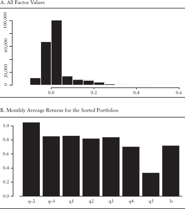
For an example of method 6, recall the discussion of the share repurchase factor from the prior companion chapter. We are interested in the extreme positive and negative values of this factor. As we see in Exhibit 12.5(A), the distribution of this factors is leptokurtic with the positive values skewed to the right and the negative values clustered in a small range. By choosing method 6 to sort this variable, we can distinguish between those values we view as extreme. The negative values are clustered so we want to distinguish among the magnitudes of those values. We accomplish this because our sorting method separates the negative values by the median of the negative values. The largest negative values form the extreme negative portfolio. The positive values are skewed to the right, so we want to differentiate between the larger from smaller positive values. When implementing portfolio method 6, we would also separate the zero values from the positive values.

The portfolio sort methodology has several advantages. The approach is easy to implement and can easily handle stocks that drop out or enter into the sample. The resulting portfolios diversify away idiosyncratic risk of individual assets and provide a way of assessing how average returns differ across different magnitudes of a factor.

The portfolio sort methodology has several disadvantages. The resulting portfolios may be exposed to different risks beyond the factor the portfolio was sorted on. In those instances, it is difficult to know which risk characteristics have an impact on the portfolio returns. Because portfolio sorts are nonparametric, they do not give insight as to the functional form of the relation between the average portfolio returns and the factor.

Next we provide three examples to illustrate how the economic intuition of the factor and cross sectional statistics can help determine the sorting methodology.

Example 1: Portfolio Sorts Based on the EBITDA/EV Factor

In the previous chapter, we introduced the EBITDA/EV factor. Panel A of Exhibit 12.1 contains the cross-sectional distribution of the EBITDA/EV factor. This distribution is approximately normally distributed around a mean of 0.1, with a slight right skew. We use method 1 to sort the variables into five portfolios (denoted by q1, …, q5) because this sorting method aligns the cross-sectional distribution of factor returns with our economic intuition that there is a linear relationship between the factor and subsequent return. In Exhibit 12.1(B), we see that there is a large difference between the equally weighted monthly returns of portfolio 1 (q1) and portfolio 5 (q5). Therefore, a trading strategy (denoted by ls in the graph) that goes long portfolio 1 and short portfolio 5 appears to produce abnormal returns.

EXHIBIT 12.1 Portfolio Sorts Based on the EBITDA/EV Factor

Example 2: Portfolios Sorts Based on the Revisions Factor

In Exhibit 12.2(A), we see that the distribution of earnings revisions is leptokurtic around a mean of about zero, with the remaining values symmetrically distributed around the peak. The pattern in this cross-sectional distribution provides insight on how we should sort this factor. We use method 3 to sort the variables into five portfolios. The firms with no change in revisions we allocate to the middle portfolio (portfolio 3). The stocks with positive revisions we sort into portfolios 1 and 2, according to the size of the revisions—while we sort stocks with negative revisions into portfolios 4 and 5, according to the size of the revisions. In Exhibit 12.2(B), we see there is the relationship between the portfolios and subsequent monthly returns. The positive relationship between revisions and subsequent returns agrees with the factor's underlying economic intuition: We expect that firms with improving earnings should outperform. The trading strategy that goes long portfolio 1 and short portfolio 5 (denoted by ls in the graph) appears to produce abnormal returns.

EXHIBIT 12.2 The Revisions Factor

Example 3: Portfolio Sorts Based on the Share Repurchase Factor

In Exhibit 12.3(A), we see the distribution of share repurchase is asymmetric and leptokurtic around a mean of zero. The pattern in this cross-sectional distribution provides insight on how we should sort this factor. We use method 6 to sort the variables into seven portfolios. We group stocks with positive revisions into portfolios 1 through 5 (denoted by q₁, …, q₅ in the graph) according to the magnitude of the share repurchase factor. We allocate stocks with negative repurchases into portfolios q−2 and q−1 where the median of the negative values determines their membership. We split the negative numbers because we are interested in large changes in the shares outstanding. In Exhibit 12.3(B), unlike the other previous factors, we see that there is not a linear relationship between the portfolios. However, there is a large difference in return between the extreme portfolios (denoted by ls in the graph). This large difference agrees with the economic intuition of this factor. Changes in the number of shares outstanding is a potential signal for the future value and prospects of a firm. On the one hand, a large increase in shares outstanding may (1) signal to investors the need for additional cash because of financial distress, or (2) that the firm may be overvalued. On the other hand, a large decrease in the number of shares outstanding may indicate that management believes the shares are undervalued. Finally, small changes in shares outstanding, positive or negative, typically do not have an impact on stock price and therefore are not significant.

EXHIBIT 12.3 The Share Repurchase Factor

Information Ratios for Portfolio Sorts

The information ratio (IR) is a statistic for summarizing the risk-adjusted performance of an investment strategy. It is defined as the ratio of the average excess return to the standard deviation of return. For actively managed equity long portfolios, the IR measures the risk-adjusted value a portfolio manager is adding relative to a benchmark.² IR can also be used to capture the risk-adjusted performance of long-short portfolios from a portfolio sorts. When comparing portfolios built using different factors, the IR is an effective measure for differentiating the performance between the strategies.

New Research on Portfolio Sorts

As we mentioned earlier in this section, the standard statistical testing procedure for portfolios sorts is to use a Student's t-test to evaluate the mean return differential between the two portfolios containing stocks with the highest and lowest values of the sorting factor. However, evaluating the return between these two portfolios ignores important information about the overall pattern of returns among the remaining portfolios.

Recent research by Patton and Timmermann³ provides new analytical techniques to increase the robustness of inference from portfolios sorts. The technique tests for the presence of a monotonic relationship between the portfolios and their expected returns. To find out if there is a systematic relationship between a factor and portfolio returns, they use the monotonic relation (MR) test to reveal whether the null hypothesis of no systematic relationship can be rejected in favor of a monotonic relationship predicted by economic theory. By MR it is meant that the expected returns of a factor should rise or decline monotonically in one direction as one goes from one portfolio to another. Moreover, Patton and Timmermann develop separate tests to determine the direction of deviations in support of or against the theory.

The authors emphasize several advantages in using this approach. The test is nonparametric and applicable to other cases of portfolios such as two-way and three-way sorts. This test is easy to implement via bootstrap methods. Furthermore, this test does not require specifying the functional form (e.g., linear) in relating the sorting variable to expected returns.