VII.11 Mathematics and Medical Statistics

David J. Spiegelhalter

1 Introduction

There are many ways in which mathematics has been applied in medicine: for example, the use of differential equations in pharmacokinetics and models for epidemics in populations; and FOURIER ANALYSIS [III.27] of biological signals. Here we are concerned with medical statistics, by which we mean collecting data about individuals and using it to draw conclusions about the development and treatment of disease. This definition may appear to be rather restrictive, but it includes all of the following: randomized clinical trials of therapies, evaluating interventions such as screening programs, comparing health outcomes in different populations and institutions, describing and comparing the survival of groups of individuals, and modeling the way in which a disease develops, both naturally and when it is influenced by an intervention. In this article we are not concerned with epidemiology, the study of why diseases occur and how they spread, although most of the formal ideas described here can be applied to it.

After a brief historical introduction, we shall summarize the varied approaches to probabilistic modeling in medical statistics. We shall then illustrate each one in turn using data about the survival of a sample of patients with lymphoma, showing how alternative “philosophical” perspectives lead directly to different methods of analysis. Throughout, we shall give an indication of the mathematical background to what can appear to be a conceptually untidy subject.

2 A Historical Perspective

One of the first uses of probability theory in the late seventeenth century was in the development of “life-tables” of mortality in order to decide premiums for annuities, and Charles Babbage’s work on life-tables in 1824 helped motivate him to design his “difference engine” (although it was not until 1859 that Scheutz’s implementation of the engine finally calculated a life-table). However, statistical analysis of medical data was a matter of arithmetic rather than mathematics until the growth of the “biometric” school founded by Francis Galton and Karl Pearson at the end of the nineteenth century. This group introduced the use of families of PROBABILITY DISTRIBUTIONS [III.71] to describe populations, as well as concepts of correlation and regression in anthropology, biology, and eugenics. Meanwhile, agriculture and genetics motivated Fisher’s huge contributions in the theory of likelihood (see below) and significance testing. Postwar statistical developments were influenced by industrial applications and a U.S.-led increase in mathematical rigor, but from around the 1970s medical research, particularly concerning randomized trials and survival analysis, has been a major methodological driver in statistics.

For around thirty years after 1945 there were many attempts to put statistical inference on a sound foundational or axiomatic basis, but no consensus could be reached. This has given rise to a widespread ecumenical perspective which makes use of a mix of statistical “philosophies” which we shall illustrate below. The somewhat uncomfortable lack of an axiomatic basis can make statistical work deeply unattractive to many mathematicians, but it provides a great stimulus to those engaged in the area.

3 Models

In this context, by a model we mean a mathematical description of a probability distribution for one or more currently uncertain quantities. Such a quantity might, for example, be the outcome of a patient who is treated with a particular drug, or the future survival time of a patient with cancer. We can identify four broad approaches to modeling—these brief descriptions make use of terms that will be covered properly in later sections.

  (i) A nonparametric or “model-free” approach that leaves unspecified the precise form for the probability distributions of interest.

 (ii) A full parametric model in which a specific form is assumed for each probability distribution, which depends on a limited number of unknown parameters.

(iii) A semi-parametric approach in which only part of the model is parametrized, while the rest is left unspecified.

(iv) A Bayesian approach in which not only is a full parametric model specified, but an additional “prior” distribution is provided for the parameters.

These are not absolute distinctions: for example, some apparently “model-free” procedures may turn out to match procedures that are derived under certain parametric assumptions.

Another complicating factor is the multiplicity of possible aims of a statistical analysis. These may include

• estimating unknown parameters, such as the mean reduction in blood pressure when giving a certain dose of a certain drug to a defined population;
• predicting future quantities, such as the number of people with AIDS in a country in ten years’ time;
• testing a hypothesis, such as whether a particular drug improves survival for a particular class of patents, or equivalently assessing the “null hypothesis” that it has no effect;
• making decisions, such as whether to provide a particular treatment in a health care system.

A common aspect of these objectives is that any conclusion should be accompanied by some form of assessment of the potential for an error having been made, and any estimate or prediction should have an associated expression of uncertainty. It is this concern for “second-order” properties that distinguishes a statistical “inference” based on probability theory from a purely algorithmic approach to producing conclusions from data.

4 The Nonparametric or “Model-Free” Approach

Now let us introduce a running example that will be used to illustrate the various approaches.

Matthews and Farewell (1985) report data on sixty-four patients from Seattle’s Fred Hutchinson Cancer Research Center who had been diagnosed with advanced-stage non-Hodgkin’s lymphoma: for each patient the information comprises their follow-up time since diagnosis, whether their follow-up ended in death, whether they presented with clinical symptoms, their stage of disease (stage IV or not), and whether a large abdominal mass (greater than 10 cm) was present. Such information has many uses. For example, we may wish to look at the general distribution of survival times, or assess which factors most influence survival, or provide a new patient with an estimate of their chance of surviving, say, five years. This is, of course, too small and limited a data set to draw firm conclusions, but it allows us to illustrate the different mathematical tools that can be used.

We need to introduce a few technical terms. Patients who are still alive at the end of data collection, or have been lost to follow-up, are said to have their survival times “censored”: all we know is that they survived beyond the last time that any data was recorded about them. We also tend to call times of death “failure” times, since the forms of analysis do not just apply to death. (This term also reflects the close connection between this area and reliability theory.)

The original approach to such survival data was “actuarial,” using the life-table techniques mentioned previously. Survival times are grouped into intervals such as years, and simple estimates are made of one’s chance of dying in an interval given that one was alive at the start of it. Historically, this probability was known as the “force of mortality,” but now it is usually called the hazard. A simple approach like this may be fine for describing large populations.

It was not until Kaplan and Meier (1958) that this procedure was refined to take into account the exact rather than the grouped survival times: with over thirty thousand citations, their paper is one of the most referenced papers in all of science. Figure 1 shows so-called Kaplan–Meier curves for the groups of patients with (n = 31) and without (n = 33) clinical symptoms at diagnosis.

These curves represent estimates of the underlying survival function, whose value at a time t is thought of as the probability that a typical patient will survive until that time. The obvious way of producing such a curve is simply to let its value at time t be the proportion of the initial sample that is still alive. However, this does not quite work, because of the censored patients. So instead, if a patient dies at time t, and if, just before time t, there are m patients still in the sample, then the value of the curve is multiplied by (m − 1)/m; and if a patient is censored then the value stays the same. (The tick marks on the curves show the censored survival times.) The set of patients alive just before time t is called the risk set and the hazard at t is estimated to be 1/m. (We are assuming that two people do not die Years since diagnosis at the same time, but it is easy to drop that assumption and make appropriate adjustments.)

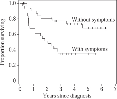
Figure 1 Kaplan–Meier nonparametric survival curves for lymphoma patients with and without clinical symptoms at diagnosis.

Although we do not assume that the actual survival curve has any particular functional form, we do need to make the qualitative assumption that the censoring mechanism is independent of the survival time. (For example, it is important that those who are about to die are not for some reason preferentially removed from the study.) We also need to provide error bounds on the curves: these can be based on a variance formula developed by Major Greenwood in 1926. (“Major” was his name rather than a title, one of the few characteristics he shared with Count Basie and Duke Ellington.)

The “true underlying survival curve” is a theoretical construct, and not something that one can directly observe. One can think of it as the survival experience that would be observed in a vast population of patients, or equivalently the expected survival for a new individual drawn at random from that population. As well as estimating these curves for the two groups of patients, we may wish to test hypotheses about them. A typical one would be that the true underlying survival curves in the two groups are precisely the same. Traditionally such “null” hypotheses are denoted H₀, and the traditional way to test them is to determine how unlikely it is that we would observe two Kaplan–Meier curves that are so far apart if H₀ were true. One can construct a summary measure, known as a test statistic, that is large if the observed curves are very different. For example, one possibility is to contrast the observed number of deaths in those with symptoms (O = 20) with the number one would have expected if H₀ were true (E = 11.9). Under the null hypothesis it turns out there is only a 0.2% chance of observing such a high discrepancy between O and E, which casts considerable doubt on the null hypothesis in this case.

When constructing intervals around estimates and testing hypotheses we require approximate probability distributions for our estimates and test statistics. From a mathematical perspective the important theory therefore concerns large-sample distributions of functions of random variables, largely developed in the early twentieth century. Theories for optimal hypothesis testing were developed by Neyman and Pearson in the 1930s: the idea is to maximize the “power” of a test to detect a difference, while at the same time making sure that the probability of wrongly rejecting a null hypothesis is less than some acceptable threshold such as 5% or 1%. This approach still finds a role in the design of randomized clinical trials.

5 Full Parametric Models

Clearly we do not actually believe that deaths can only occur at the previously observed survival times shown in the Kaplan–Meier curve, so it seems reasonable to investigate a fairly simple functional form for the true survival function. That is, we assume that the survival function belongs to some natural class of functions, each of which can be fully parametrized by a small number of parameters, collectively denoted by θ. It is θ that we are trying to discover (or rather estimate with a reasonable degree of confidence). If we can do so, then the model is fully specified and we can even extrapolate a certain amount beyond the observed data. We first relate the survival function and the hazard, and then illustrate how observed data can be used to estimate θ in a simple example.

We assume that an unknown survival time has a probability density p(t|θ); without getting into technical details, this essentially corresponds to assuming that p(t|θ) dt is the probability of dying in a small interval t to t + dt. Then the survival function, given a particular value of θ, is the probability of surviving beyond t: we denote it by S(t|θ). To calculate it, we integrate the probability density over all times greater than t. That is,

S(t|θ) = p(x|θ) dx = 1 − p(x|θ) dx.

From this and THE FUNDAMENTAL THEOREM OF CALCULUS [I.3 §5.5] it follows that p(t|θ) = −dS(t|θ)/dt. The hazard function h(t|θ) dt is the risk of death in the small interval t to t+ dt, conditional on having survived to time t. Using the laws of elementary probability we find that

h(t|θ) = p(t|θ)/S(t|θ).

For example, suppose we assume an exponential survival function with mean survival time θ, so that the probability of surviving beyond time t is S(t|θ) = e^-t/θ. The density is p(t|θ) = e^-t/θ/θ. Therefore, the hazard function is a constant h(t|θ) = 1/θ, so that 1/θ represents the mortality rate per unit of time. For instance, were the mean postdiagnosis survival to be θ = 1000 days, an exponential model would imply a constant 1/1000 risk of dying each day, regardless of how long the patient had already survived after diagnosis. More complex parametric survival functions allow hazard functions that increase, decrease, or have other shapes.

When it comes to estimating θ we need Fisher’s concept of likelihood. This takes the probability distribution p (t|θ) but considers it as a function of θ rather than t, and hence for observed t allows us to examine plausible values of θ that “support” the data. The rough idea is that we multiply together the probabilities (or probability densities) of the observed events, assuming the value of θ. In survival analysis, observed and censored failure times make different contributions to this product: an observed time t contributes p(t|θ), while a censored time contributes S(t|θ). If, for example, we assume that the survival function is exponential, then an observed failure time contributes p(t|θ) = e^-t/θ/θ, and a censored time contributes S(t|θ) = e^−t/θ. Thus, in this case the likelihood is

Here “Obs” and “Cens” indicate the sets of observed and censored failure times. We denote their sizes by n_o and n_c, respectively, and we denote the total follow-up time Σ_it_i by T. For the group of thirty-one patients presenting with symptoms we have n_o = 20 and T = 68.3 years: figure 2 shows both the likelihood and its logarithm

LL(θ)= -T|θ-n_O log θ.

We note that the vertical axis for the likelihood is unlabeled since only relative likelihood is important. A maximum-likelihood estimate (MLE) finds parameter values that maximize this likelihood or equivalently the log-likelihood. Taking derivatives of LL(θ) and equating to 0 reveals that = T| n_Obs = 3.4 years, which is the total follow-up time divided by the number of failures. Intervals around MLEs may be derived by directly examining the likelihood function, or by making a quadratic approximation around the maximum of the log-likelihood.

Figure 2 Likelihood and log-likelihood for mean survival time θ for lymphoma patients presenting with clinical symptoms.

Figure 3 shows the fitted exponential survival curves: loosely, we have carried out a form of curve fitting by selecting the exponential curves that maximize the probability of the observed data. Visual inspection suggests the fit may be improved by investigating a more flexible family of curves such as the Weibull distribution (a distribution widely used in reliability theory): to compare how well two models fit the data, one can compare their maximized likelihoods.

Fisher’s concept of likelihood has been the foundation for most current work in medical statistics, and indeed statistics in general. From a mathematical perspective there has been extensive development relating the large-sample distributions of MLEs to the second derivative of the log-likelihood around its maximum, which forms the basis for most of the outputs of statistical packages. Unfortunately, it is not necessarily straightforward to scale up the theory to deal with multidimensional parameters. First, as likelihoods become more complex and contain increasing numbers of parameters, the technical problems of maximization increase. Second, the recurring difficulty with likelihood theory remains that of “nuisance parameters,” in which a part of the model is of no particular interest and yet needs to be accounted for. No generic theory has been developed, and instead there is a some-what bewildering variety of adaptations of standard likelihood to specific circumstances, such as conditional likelihood, quasi-likelihood, pseudo-likelihood, extended likelihood, hierarchical likelihood, marginal likelihood, profile likelihood, and so on. Below we consider one extremely popular development, that of partial likelihood and the Cox model.

Figure 3 Fitted exponential survivalcurves for lymphoma patients.

6 A Semi-Parametric Approach

Clinical trials in cancer therapy were a major motivating force in developing survival analysis—in particular, trials to assess the influence of a treatment on survival while taking account of other possible risk factors. In our simple lymphoma data set we have three risk factors, but in more realistic examples there will be many more. Fortunately, Cox (1972) showed that it was possible both to test hypotheses and to estimate the influence of possible risk factors, without having to go the whole way and specify the full survival function on the basis of possibly limited data.

The Cox regression model is based on assuming a hazard function of the form

h(t|θ) = h₀(t)e^ß.x.

Here h₀(t) is a baseline hazard function and β is typically a column vector of regression coefficients that measure the influence of a vector of risk factors x on the hazard. (The expression β · x denotes the scalar product of β and x.) The baseline hazard function corresponds to the hazard function of an individual whose risk factor vector is x = 0, since then e^β·x = 1. More generally, we see that an increase of one unit in a factor x_j will multiply the hazard by a factor e^β_j, for which reason this is known as the “proportional hazards” regression model. It is possible to specify a parametric form for h₀(t), but remarkably it turns out to be possible to estimate the terms of β without specifying the form of the h₀, if we are willing to consider the situation immediately before a particular failure time. Again we construct a risk set, and the chance of a particular patient failing, given the knowledge that someone in the risk set fails, provides a term in a likelihood. This is known as a “partial” likelihood since it ignores any possible information in the times between failures.

When we fit this model to the lymphoma data we find that our estimate of β for the patients with symptoms is 1.2: easier to interpret is its exponent e^1.2 = 3.3, which is the proportional increase in hazard associated with presenting with symptoms. We can estimate error bounds of 1.5–7.3 around this estimate, so we can be confident that the risk of a patient who presents with symptoms will die at any stage following diagnosis is substantially higher than that of a patient who does not present with symptoms, all other factors in the model being kept constant.

A huge literature has arisen from this model, dealing with errors around estimates, different censoring patterns, tied failure times, estimating the baseline survival, and so on. Large-sample properties were rigorously established only after the method came into routine use, and have made extensive use of the theory of stochastic counting processes: see, for example, Andersen et al. (1992). These powerful mathematical tools have enabled the theory to be expanded to deal with the general analysis of sequences of events, while allowing for censoring and multiple risk factors that may depend on time.

Cox’s 1972 paper has over twenty thousand citations, and its importance to medicine is reflected in his having been awarded the 1990 Kettering Prize and Gold Medal for Cancer Research.

7 Bayesian Analysis

Bayes’s theorem is a basic result in probability theory. It states that, for two random quantities t and θ,

p(θ|t) = p(t|θ)p(θ)/p(t).

In itself this is a very simple fact, but when θ represents parameters in a model, the use of this theorem represents a different philosophy of statistical modeling. The major step in using Bayes’s theorem for inference is in considering parameters as RANDOM VARIABLES [III.71 §4] with probability distributions and therefore making probabilistic statements about them. For example, in the Bayesian framework one could express one’s uncertainty about a survival curve by saying that one had assessed that the probability that the mean survival time was greater than three years was 0.90. To make such an assessment, one can combine a “prior” distribution p(θ) (a distribution representing the relative plausibility of different values of θ before you look at the data) with a likelihood p(t|θ) (how likely you were to observe the data t with that value of θ) and then use Bayes’s theorem to provide a “posterior” distribution p(θ|t) (a distribution representing the relative plausibility of different values of θ after you look at the data).

Put in this way Bayesian analysis appears to be a simple application of probability theory, and for any given choice of prior distribution that is exactly what it is. But how do you choose the prior distribution? You could use evidence external to the current study, or even your own personal judgment. There is also an extensive literature on attempts to produce a toolkit of “objective” priors to use in different situations. In practice you need to specify the prior distribution in a way that is convincing to others, and this is where the subtlety arises.

As a simple example, suppose that previous studies of lymphoma had suggested that mean survival times of patients presenting with clinical symptoms probably lie between three and six years, with values of around four years being most plausible. Then it seems reasonable not to ignore such evidence when drawing conclusions for future patients, but rather to combine it with the evidence from the thirty-one patients in the current study. We could represent this external evidence by a prior distribution for θ with the form given in figure 4. When combined with the likelihood (taken from figure 2(a)), this gives rise to the posterior distribution shown. For this calculation, the functional form of the prior is assumed to be that of the inverse-Gamma distribution, which happens to make the mathematics of dealing with exponential likelihoods particularly straightforward, but such simplifications are not necessary if one is using simulation methods for deriving posterior distributions.

It can be seen from figure 4 that the external evidence has increased the plausibility of higher survival times. By integrating the posterior distribution above three years, we find that the posterior probability that the mean survival is greater than three years is 0.90.

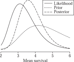
Figure 4 Prior, likelihood, and posterior distributions for mean survival time θ for patients presenting with symptoms. The posterior distribution is a formal compromise between the likelihood, which summarizes the evidence in the data alone, and the prior distribution, which summarizes external evidence that suggested longer survival times.

Likelihoods in Bayesian models need to be fully parametric, although semi-parametric models such as the Cox model can be approximated by high-dimensional functions of nuisance parameters, which then need to be integrated out of the posterior distributions. Difficulties with evaluating such integrals held up realistic applications of Bayesian analysis for many years, but now developments in simulation approaches such as Markov chain Monte Carlo (MCMC) methods have led to a startling growth in practical Bayesian analyses. Mathematical work in Bayesian analysis has mainly focused on theories of objective priors, large-sample properties of posterior distributions, and dealing with hugely multivariate problems and the necessary high-dimensional integrals.

8 Discussion

The preceding sections have given some idea of the tangled conceptual issues that underlie even routine medical statistical analysis. We need to distinguish a number of different roles for mathematics in medical statistics—the following are a few examples.

Individual applications: here the use of mathematics is generally quite limited, since extensive use is made of software packages, which can fit a wide variety of models. In nonstandard problems, algebraic or numerical maximization of likelihoods may be necessary, or developing MCMC algorithms for numerical integration.

Derivation of generic methods: these can then be implemented in software. This is perhaps the most widespread mathematical work, which requires extensive use of probability theory on functions of random variables, particularly using large-sample arguments.

Proof of properties of methods: this requires the most sophisticated mathematics, which concerns topics such as the convergence of estimators, or the behavior of Bayesian methods under different circumstances.

Medical applications continue to be a driving force in the development of new methods of statistical analysis, partly because of new sources of high-dimensional data from areas such as bioinformatics, imaging, and performance monitoring, but also because of the increasing willingness of health policy makers to use complex models: this has the consequence of focusing attention on analytic methods and the design of studies for checking, challenging, and refining such models.

Nevertheless, it may appear that rather limited mathematical tools are required in medical statistics, even for those engaged in methodological research. This is compensated for by the fascinating and continuing debate over the underlying philosophy of even the most common statistical tools, and the consequent variety of approaches to apparently simple problems. Much of this debate is hidden from the routine user. Regarding the appropriate role of mathematical theory in statistics, we can do no better than quote David Cox in his 1981 Presidential Address to the Royal Statistical Society (Cox 1981):

Lord Rayleigh defined applied mathematics as being concerned with quantitative investigation of the real world “neither seeking nor evading mathematical difficulties.” This describes rather precisely the delicate relation that ideally should hold between mathematics and statistics. Much fine work in statistics involves minimal mathematics; some bad work in statistics gets by because of its apparent mathematical content. Yet it would be harmful for the development of the subject for there to be widespread an anti-mathematical attitude, a fear of powerful mathematics appropriately deployed.

Further Reading

Andersen, P. K., O. Borgan, R. Gill, and N. Keiding. 1992. Statistical Models Based on Counting Processes. New York: Springer.

Cox, D. R. 1972. Theory and general principle in statistics. Journal of the Royal Statistical Society A144:289–97.

——. 1981. Regression models and life-tables (with discussion). Journal of the Royal Statistical Society B34:187–220.

Kaplan, E. L., and P. Meier. 1958. Nonparametric estimation from incomplete observations. Journal of the American Statistical Association 53:457–81.

Matthews, D. E., and V. T. Farewell. 1985. Using and Understanding Medical Statistics. Basel: Karger.