---

IV.14 Dynamics

Bodil Branner

---

1 Introduction

Dynamical systems are used to describe the way systems evolve in time, and have their origin in the laws of nature that NEWTON [VI. 14] formulated in Principia Mathematica (1687). The associated mathematical discipline, the theory of dynamics, is closely related to many parts of mathematics, in particular analysis, topology, measure theory, and combinatorics. It is also highly influenced and stimulated by problems from the natural sciences, such as celestial mechanics, hydrodynamics, statistical mechanics, meteorology, and other parts of mathematical physics, as well as reaction chemistry, population dynamics, and economics.

Computer simulations and visualizations play an important role in the development of the theory; they have changed our views about what should be considered typical, rather than special and atypical.

There are two main branches of dynamical systems: continuous and discrete. The main focus of this paper will be holomorphic dynamics, which concerns discrete dynamical systems of a special kind. These systems are obtained by taking a HOLOMORPHIC FUNCTION [I.3 §5.6] f defined on the complex numbers and applying it repeatedly. An important example is when f is a quadratic polynomial.

1.1 Two Basic Examples

It is interesting to note that both types of dynamical system, continuous and discrete, can be well illustrated by examples that date back to Newton.

(i) The N-body problem models the motion in the solar system of the sun and N - 1 planets, and does so in terms of differential equations. Each body is represented by a single point, namely its center of mass, and the motion is determined by Newton’s universal law of gravitation— also called the inverse square law. This says that the gravitational force between two bodies is proportional to each of their masses and inversely proportional to the square of the distance between them. Let r_i denote the position vector of the ith body, m_i its mass, and the universal gravitational constant. Then the force on the ith body due to the jth has magnitude gm_im_j/||r_j-r_i||², and its direction is along the line from r_i to r_j. We can work out the total force on the ith body by adding up all these forces for j ≠ i Since a unit vector in the direction from r_i to r_j is (r_j-r_i)/||r_j-r_i||, we obtain a force of

(There is a cube on the bottom rather than a square in order to compensate for the magnitude of r_j - r_i.) A solution to the N-body problem is a set of differentiable vector functions (r₁ (t), . . . , rN(t)), depending on time t, that satisfy the N differential equations

which result from Newton’s second law, which states that force = mass × acceleration.

Newton was able to solve the two-body problem explicitly. By neglecting the influence of other planets, he derived the laws formulated by Johannes Kepler, which describe how each planet moves in an elliptic orbit around the sun. However, the jump to N > 2 makes an enormous difference to the complication of the problem: except in very special cases, the system of equations can no longer be solved explicitly (see THE THREE-BODY PROBLEM [V.33]). Nevertheless, Newton’s equations are of great practical importance when it comes to guiding satellites and other space missions.

(ii) NEWTON’S METHOD [II.4§2.3] for solving equations is quite different and does not involve differential equations. We consider a differentiable function f of one real variable and wish to determine a zero of f, that is, a solution to the equation f (x) = 0. Newton’s idea was to define a new function:

To put this more geometrically, N_f(x) is the x-coordinate of the point where the tangent line to the graph y = f(x) at the point (x, f(x)) crosses the x-axis. (If f′(x) = 0, then this tangent line is horizontal and N_f(x) is not defined.)

Under many circumstances, if x is close to a zero of f, then N_f(x) is significantly closer. Therefore, if we start with some value x₀ and form the sequence obtained by repeated application of N_f, that is, the sequence x₀, x₁, x₂ , . . . , where x₁ = N_f(x₀), x₂ = N_f(x₁), and so on, we can expect that this sequence will converge to a zero of f. And this is true: if the initial value x₀ is sufficiently close to a zero, then the sequence does indeed converge toward that zero, and does so extremely quickly, basically doubling the number of correct digits in each step. This rapid convergence makes Newton’s method very useful for numerical computations.

1.2 Continuous Dynamical Systems

We can think of a continuous dynamical system as a system of first-order differential equations, which determine how the system evolves in time. A solution is called an orbit or trajectory, and is parametrized by a number t, which one usually thinks of as time, that takes real values and varies continuously: hence the name “continuous” dynamical system. A periodic orbit of period T is a solution that repeats itself after time T, but not earlier.

The differential equation x″(t) = -x(t) is of second order, but it is nevertheless a continuous dynamical system because it is equivalent to the system of two first-order differential equations x′₁ (t) = x₂(t) and x′₂ (t) = -x₁(t). In a similar way, the system of differential equations of the N-body problem can be brought into standard form by introducing new variables. The equations are equivalent to a system of 6N first-order differential equations in the variables of the position vectors r_i = (x_i1, x_i2, x_i3) and the velocity vectors r′_i = (y_i1, y_i2, y_i3). Thus, the N-body problem is a good example of a continuous dynamical system.

In general, if we have a dynamical system consisting of n equations, then we can write the ith equation in the form

or alternatively we can write all the equations at once in the form x′(t) = f(x(t)), where x(t) is the vector (x₁(t) , . . . ,x_n(t)) and f = (f₁ , . . . , f_n) is a function from ⁿ to ⁿ. Note that f is assumed not to depend on t. If it does, then the system can be brought into standard form by adding the variable x_n+1 = t and the differential equation x′_n+1(t) = 1, which increases the dimension of the system from n to n + 1.

The simplest systems are linear ones, where f is a linear map: that is, f(x) is given by Ax for some constant n × n matrix A. The system above, x′₁(t) = x₂(t) and x′₂(t), is an example of a linear system. Most systems, however, including the one for the N-body problem, are nonlinear. If the function f is “nice” (for instance, differentiable), then uniqueness and existence of solutions are guaranteed for any initial point x₀. That is, there is exactly one solution that passes through the point x₀ at time t = 0. For example, in the N-body problem there is exactly one solution for any given set of initial position vectors and initial velocity vectors. It also follows from uniqueness that any pair of orbits must either coincide or be totally disjoint. (Bear in mind that the word “orbit” in this context does not mean the set of positions of a single point mass, but rather the evolution of the vector that represents all the positions and velocities of all the masses.)

Although it is seldom possible to express solutions to nonlinear systems explicitly, we know that they exist, and we call the dynamical system deterministic since solutions are completely determined by their initial conditions. For a given system and given initial conditions it is therefore theoretically possible to predict its entire future evolution.

1.3 Discrete Dynamical Systems

A discrete dynamical system is a system that evolves in jumps: “time,” in such a system, is best represented by an integer rather than a real number. A good example is Newton’s method for solving equations. In this instance, the sequence of points we saw earlier, x₀, x₁ , . . . ,x_k , . . . , where x_k = N_f(x_k-1), is called the orbit of x₀. We say that it is obtained by iteration of the function N_f, i.e., by repeated application of the function.

This idea can easily be generalized to other mappings F : X → X, where X could be the real axis, an interval in the real axis, the plane, a subset of the plane, or some more complicated space. The important thing is that the output F(x) of any input x can be used as the next input. This guarantees that the orbit of any x₀ in X is defined for all future times. That is, we can define a sequence, x₀,x₁ , . . . ,x_k , . . . , where x_k = F(x_k-1) for every k. If the function F has an inverse F^-1, then we can iterate both forwards and backwards and obtain the full orbit of x₀ as the bi-infinite sequence . . . ,x_-2,x_-1,x₀,x₁,x₂ , . . . , where x_k = F(x_k-1) and, equivalently, x_k-1 = F^-1(x_k), for all integer values.

The orbit of x₀ is periodic of period k if it repeats itself after time k, but not earlier, i.e., if x_k = x₀, but x_j x₀ for j = 1 , . . . ,k - 1. The orbit is called pre-periodic if it is eventually periodic, in other words if there exist 1 and k 1 such that x is periodic of period k, but none of the x_j for 0 j < are periodic. The notion of pre-periodicity has no counterpart in continuous dynamics.

A discrete dynamical system is deterministic, since the orbit of any given initial point x₀ is completely determined once you know x₀

1.4 Stability

The modern theory of dynamics was greatly influenced by the work of POINCARÉ [VI.61], and in particular by his prize-winning memoir on the three-body problem, succeeded by three more elaborate volumes on celestial mechanics, all from the late nineteenth century. The memoir was written in response to a competition where one of the proposed problems concerned stability of the solar system. Poincaré introduced the so-called restricted three-body problem, where the third body is assumed to have an infinitely small mass: it does not influence the motion of the other two bodies but it is influenced by them. Poincaré’s work became the prelude to topological dynamics, which focuses on topological properties of solutions to dynamical systems and takes a qualitative approach to them.

Of special interest is the long-term behavior of a system. A periodic orbit is called stable if all orbits through points sufficiently close to it stay close to it at all future times. It is called asymptotically stable if all sufficiently close orbits approach it as time tends to infinity. Let us illustrate this by two linear examples in discrete dynamics. For the real function F(x) = -x, all points have a periodic orbit: 0 has period 1 and all other x have period 2. Every orbit is stable, but none is asymptotically stable. The real function G(x) = x has only one periodic orbit, namely 0. Since G(0) = 0, this orbit has period 1, and we call it a fixed point. If you take any number and repeatedly divide it 2, then the resulting sequence will approach 0, so the fixed point 0 is asymptotically stable.

One of the methods introduced by Poincaré during his study of the three-body problem was a reduction from a continuous dynamical system, in dimension n, say, to an associated discrete dynamical system, a mapping in dimension n - 1. The idea is as follows. Suppose we have a periodic orbit of period T > 0 in some continuous system. Choose a point x₀ on the orbit and a hypersurface Σ through x₀, for instance part of a hyperplane, such that the orbit cuts through Σ at x₀. For any point in Σ that is sufficiently close to x₀, one can follow its orbit around and see where it next intersects Σ. This defines a transformation, known as the Poincaré map, which takes the original point to the next point of intersection of its orbit with Σ. It follows from the fact that dynamical systems have unique solutions that every Poincaré map is injective in the neighborhood of x₀ (within Σ) for which the Poincaré map is defined. One can perform both forwards and backwards iterations. Note that the periodic orbit of x₀ in the continuous system is stable (respectively, asymptotically stable) exactly when the fixed point x₀ of the Poincaré map in the discrete system is stable (respectively, asymptotically stable).

1.5 Chaotic Behavior

The notion of chaotic dynamics arose in the 1970s. It has been used in different settings, and there is no single definition that covers all uses of the term. However, the property that best characterizes chaos is the phenomenon of sensitive dependence on initial conditions. Poincaré was the first to observe sensitivity to initial conditions in his treatment of the three-body problem.

Instead of describing his observations let us look at a much simpler example from discrete dynamics. Take as a dynamical space X the half-open unit interval [0, 1), and let F be the function that doubles a number and reduces it modulo 1. That is, F(x) = 2x when 0 x < and F(x) = 2x - 1 when x < 1. Let x₀ be a number in X and let its iterates be x₁ = F(x₀), x² = F(x₁), and so on. Then x_k is the fractional part of 2^kx₀. (The fractional part of a real number t is what you get when you subtract the largest integer less than t.)

A good way to understand the behavior of the sequence x₀, x₁, x₂,. . . of iterates is to consider the binary expansion of x₀. Suppose, for example, that this begins 0.110100010100111 . . . . To double a number when it is written in binary, all you have to do is shift every digit to the left (just as one does in the decimal system when multiplying by 10). So 2x₀ will have a binary expansion that begins 1.10100010100111 . . . . To obtain F(x ₀), we have to take the fractional part of this, which we do by subtracting the initial 1. This gives us x₁ = 0.10100010100111 . . . . Repeating the process we find that x₂ = 0.0100010100111 . . . , x₃ = 0.100010100111 . . . , and so on. (Notice that when we calculated x₃ from x₂ there was no need to subtract 1, since the first digit after the “decimal point” was a 0.) Now consider a different choice of initial number, = 0.110100010110110 . . . . The first nine digits after the decimal point are the same as the first nine digits of x₀, so is very close to x₀. However, if we apply F ten times to x₀ and , then their respective eleventh digits have shifted leftwards and become the first digits of x₁₀ = 0.00111 . . . and = 0.10110 . . . . These two numbers differ by almost , so they are not at all close.

In general, if we know x₀ to an accuracy of k binary digits and no more, then after k iterations of the map F we have lost all information: x_k could lie anywhere in the interval [0, 1). Therefore, even though the system is deterministic, it is impossible to predict its long-term behavior without knowing x₀ with perfect accuracy.

This is true in general: it is impossible to make long-term predictions in any part of a dynamical system that shows sensitivity to initial conditions unless the initial conditions are known exactly. In practical applications this is never the case. For instance, when applying a mathematical model to perform weather forecasts, one does not know the initial conditions exactly, and this is why reliable long-term forecasting is impossible.

Sensitivity is also important in the notion of so-called strange attractors. A set A is called an attractor if all orbits that start in A stay in A and if all orbits through nearby points get closer and closer to A. In continuous systems, some simple sets that can be attractors are equilibrium points, periodic orbits (limit cycles), and surfaces such as a torus. In contrast to these examples, strange attractors have both complicated geometry and complicated dynamics: the geometry is fractal and the dynamics sensitive. We shall see examples of fractals later on.

The best-known strange attractor is the Lorenz attractor. In the early 1960s, the meteorologist Edward N. Lorenz studied a three-dimensional continuous dynamical system that gave a simplified model of heat flow. While doing so, he noticed that if he restarted his computer with its initial conditions chosen as the output of an earlier calculation, then the trajectory started to diverge from the one he had previously observed. The explanation he found was that the computer used more precision in its internal calculations than it showed in its output. For this reason, it was not immediately apparent that the initial conditions were in fact very slightly different from before. Because the system was sensitive, this tiny difference eventually made a much bigger difference. He coined the poetic phrase “the butterfly effect” to describe this phenomenon, suggesting that a small disturbance such as a butterfly flickering its wings could in time have a dramatic effect on the long-term evolution of the weather and trigger a tornado thousands of miles away. Computer simulations of the Lorenz system indicate that solutions are attracted to a complicated set that “looks like” a strange attractor. The question of whether it actually was one remained open for a long time. It is not obvious how trustworthy computer simulations are when one is studying sensitive systems, since the computer rounds off the numbers in each step. In 1998 Warwick Tucker gave a computer-assisted proof that the Lorenz attractor is in fact a strange attractor. He used interval arithmetic, where numbers are represented by intervals and estimates can be made precise.

For topological reasons, sensitivity to initial conditions is possible for continuous dynamical systems only when the dimension is at least 3. For discrete systems where the map F is injective, the dimension must be at least 2. However, for noninjective mappings, sensitivity can occur for one-dimensional systems, as we saw with the example given earlier. This is one of the reasons that discrete one-dimensional dynamical systems have been intensively studied.

1.6 Structural Stability

Two dynamical systems are said to be topologically equivalent if there is a homeomorphism (a continuous map with continuous inverse) that maps the orbits of one system onto the orbits of the other, and vice versa. Roughly speaking, this means that there is a continuous change of variables that turns one system into the other.

As an example, consider the discrete dynamical system given by the real quadratic polynomial F(x) = 4x(1 - x). Suppose we were to make the substitution y = -4x + 2. How could we describe the system in terms of y? Well, if we apply F, then we change x to 4x(1 - x), which means that y = -4x + 2 changes F(x) to -4F(x) + 2 = -16x(1 - x) + 2. But

-16x(1 - x) + 2 = 16x² - 16x + 2

= (-4x + 2)² - 2

= y² - 2.

Therefore, the effect of applying the polynomial function F to x is to apply a different polynomial function to y, namely Q(y) = y² - 2. Since the change of variables from x to -4x + 2 is continuous and invertible, one says that the functions F and Q are conjugate.

Because F and Q are conjugate, the orbit of any x₀ under F becomes, after the change of variables, the orbit of the corresponding point y₀ = -4x₀ + 2 under Q. That is, for every k we have y_k = -4x_k + 2. The two systems are topologically equivalent: if you want to understand the dynamics of one of them, you can if you study the other, since its dynamics will be qualitatively the same.

For continuous dynamical systems the notion of equivalence is slightly looser in that we allow a homeomorphism between two topologically equivalent systems to map one orbit onto another without respecting the exact time evolution, but for discrete dynamical systems we must demand that the time evolution is respected as in the example above: in other words, we insist on conjugacy.

The term dynamical system was coined by Stephen Smale in the 1960s and has taken off since then. Smale evolved the theory of robust systems, also named structurally stable systems, a notion that was introduced in the 1930s by Alexander A. Andronov and Lev S. Pontryagin. A dynamical system is called structurally stable if all systems sufficiently close to it, belonging to some specified family of systems, are in fact topologically equivalent to it. We say that they all have the same qualitative behavior. An example of the kind of family one might consider is the set of all real quadratic polynomials of the form x² + a. This family is parametrized by a, and the systems close to a given polynomial x² + a₀ are all the polynomials x² + a for which a is close to a₀. We shall return to the question of structural stability when we discuss holomorphic dynamics later.

If a family of dynamical systems parametrized by a variable a is not structurally stable, it may still be that the system with parameter a₀ is topologically equivalent to all systems with parameter a in some region that contains a₀. A major goal of research into dynamics is to understand not just the qualitative structure of each system in the family, but also the structure of the parameter space, that is, how it is divided up into such regions of stability. The boundaries that separate these regions form what is called the bifurcation set: if a₀ belongs to this set, then there will be parameters a arbitrarily close to a₀ for which the corresponding system has a different qualitative behavior.

A description and classification of structurally stable systems and a classification of possible bifurcations is not within reach for general dynamical systems. However, one of the success stories in the subject, holomorphic dynamics, studies a special class of dynamical systems for which many of these goals have been attained. It is time to turn our attention to this class.

2 Holomorphic Dynamics

Holomorphic dynamics is the study of discrete dynamical systems where the map to be iterated is a HOLOMORPHIC FUNCTION [I.3 §5.6] of the COMPLEX NUMBERS [I.3 §1.5]. Complex numbers are typically denoted by z. In this article, we shall consider iterations of complex polynomials and rational functions (that is, functions like (z² + 1)/(z³ + 1) that are ratios of polynomials), but much of what we shall say about them is true for more general holomorphic functions, such as EXPONENTIAL [III.25] and TRIGONOMETRIC [III.92] functions.

Whenever one restricts attention to a special kind of dynamical system, there will be tools that are specially adapted to that situation. In holomorphic dynamics these tools come from complex analysis. When we concentrate on rational functions, there are more special tools, and if we restrict further to polynomials, then there are yet others, as we shall see.

Why might one be interested in iterating rational functions? One answer arose in 1879, when CAYLEY [VI.46] had the idea of trying to find roots of complex polynomials by extending Newton’s method, which we discussed in the introduction, from real numbers to complex numbers. Given any polynomial P, the corresponding Newton function N_P is a rational function, given by the formula

To apply Newton’s method, one iterates this rational function.

The study of the iteration of rational functions flourished at the beginning of the twentieth century, thanks in particular to work of Pierre Fatou and Gaston Julia (who independently obtained many of the same results). Part of their work concerned the study of the local behavior of functions in the neighborhoods of a fixed point. But they were also concerned about global dynamical properties and were inspired by the theory of so-called normal families, then recently established by Paul Montel. However, research on holomorphic dynamics almost came to a stop around 1930, because the fractal sets that lay behind the results were so complicated as to be almost beyond imagination. The research came back to life in around 1980 with the vastly extended calculating powers of computers, and in particular the possibility of making sophisticated graphic visualizations of these fractal sets. Since then, holomorphic dynamics has attracted a lot of attention. New techniques continue to be developed and introduced.

To set the scene, let us start by looking at one of the simplest of polynomials, namely z².

2.1 The Quadratic Polynomial z²

The dynamics of the simplest quadratic polynomial, Q₀(z) = z², plays a fundamental role in the understanding of the dynamics of any quadratic polynomial. Moreover, the dynamical behavior of Q₀ can be analyzed and understood completely.

If z = re^iθ, then z² = r²e^2iθ, so squaring a complex number squares its modulus and doubles its argument. Therefore, the unit circle (the set of complex numbers of modulus 1) is mapped by Q₀ to itself, while a circle of radius r < 1 is mapped onto a circle closer to the origin, and a circle of radius r > 1 is mapped onto a circle farther away.

Let us look more closely at what happens to the unit circle. A typical point in the circle, e^iθ, can be parametrized by its argument θ, which we can take to lie in the interval [0, 2π). When we square this number, we obtain e^2iθ, which is parametrized by the number 2θ if 2θ < 2π, but if 2θ 2π, then we subtract 2π so that the argument, 2θ - 2π, still lies in [0 , 2π). This is strongly reminiscent of the dynamical system we considered in section 1.5. In fact, if we replace the argument θ by its modified argument θ/2π, which amounts to writing e^2πiθ instead of e^iθ, then it becomes exactly the same system. Therefore, the behavior of z² on the unit circle is chaotic.

As for the rest of the complex plane, the origin is an asymptotically stable fixed point, Q₀(0) = 0. For any point z₀ inside the unit circle the iterates z_k converge to 0 as k tends to infinity. For any point z₀ outside the unit circle the distance |z_k| between the iterates z_k and the origin tends to infinity as k tends to infinity. The set of initial points z₀ with bounded orbit is equal to the closed unit disk, i.e., all points for which |z₀| 1. Its boundary, the unit circle, divides the complex plane into two domains with qualitatively different dynamical behavior.

Some orbits of Q₀ are periodic. In order to determine which ones, we first notice that the only possibility outside the unit circle is the fixed point at the origin, since all other points, when you repeatedly square them, either get steadily closer and closer to the origin, or get steadily farther and farther away. So now let us look at the unit circle, and consider the point e^2πiθ₀, with modified argument θ₀. If this point is periodic with period k, we must have 2^kθ₀ = θ₀(mod 1): that is, (2^k - 1)θ₀ must be an integer. Because of this, it is convenient to parametrize a point on the unit circle by its modified argument. From now on, when we say “the point θ,” we shall mean the point e^2πiθ, and when we say “argument” we shall mean modified argument.

We have just established that the point θ is periodic with period k only if(2^k 1)θ is an integer. It follows that there is one point of period 1, namely θ₀ = 0. There are two points of period 2, forming one orbit, namely . There are six points for period 3, forming two orbits, namely and . (At each stage, we double the number we have, and subtract 1 if that is needed to get us back into the interval [0, 1).) The points of period 4 are fractions with denominator 15, but the converse is not true: the fractions = and = have the lower period 2. The periodic points on the unit circle are dense in the unit circle, meaning that arbitrarily close to any point is a periodic point. This follows from the observation that all repeating binary expansions, such as 0.1100011000110001100011000 . . . are periodic, and any finite sequence of 0s and 1s is the start of a repeating sequence. One can, in fact, show that the periodic points on the unit circle are exactly the points whose argument is a fraction p/q in [0, 1) with q odd. Any fraction with even denominator can be written in the form p/(2q) for some odd number q. After iterations, such a fraction will land on a periodic point, so the initial point is pre-periodic. Points with rational argument in [0, 1) have a finite orbit, while points with irrational argument have an infinite orbit. The reason for taking modified arguments is now justified: the behavior of the dynamics depends on whether θ₀ is rational or irrational.

When θ₀ is irrational its orbit may or may not be dense in [0, 1). This is another fact that is easy to see if one considers binary expansions. For instance, a very special example of a θ₀ with a dense orbit is given by the binary expansion

θ₀ = 0.0100011011000001010011100101110111 . . . ,

where one obtains this expansion by simply listing all finite binary sequences in turn: first the blocks of length one, 0 and 1, then the blocks of length two, 00, 01, 10, and 11, and so on. When we iterate, this binary expansion shifts to the left and all possible finite sequences appear at some time or another at the beginning of some iterate θ_k.

2.2 Characterization of Periodic Points

Let z₀ be a fixed point of a holomorphic map F. How do the iterates of points near z₀ behave? The answer depends crucially on a number ρ, called the multiplier of the fixed point, which is defined to be F´ (z₀). To see why this is relevant, notice that if z is very close to z₀, then F(z) is, to a first-order approximation, equal to F(z₀) + F´(z₀)(z - z₀) = z₀ + ρ(z - z₀). Thus, when you apply F to a point near z₀, its difference from z₀ approximately multiplies by ρ. If |ρ| < 1, then nearby points will get closer to z₀, in which case z₀ is called an attracting fixed point. If ρ = 0, then this happens very quickly and z₀ is called super-attracting. If |ρ| > 1, then nearby points get farther away and z₀ is called repelling. Finally, if |ρ| = 1, then one says that z₀ is indifferent.

If z₀ is indifferent, then its multiplier will take the form ρ = e^2πiθ, and near z₀ the map F will be approximately a rotation about z₀ by an angle of 2πθ. The behavior of the system depends very much on the precise value of θ. We call the fixed point rationally or irrationally indifferent if θ is rational or irrational, respectively. The dynamics is not yet completely understood in all irrational cases.

A periodic point z₀ of period k will be a fixed point of the kth iterate F^k = F ο. . ο F of F. For this reason we define its multiplier by ρ = (F^k)´(z₀). It follows from the chain rule that

and therefore that the derivative of F^k is the same at all points of the periodic orbit. This formula also implies that a super-attracting periodic orbit must contain a critical point (that is, a point where the derivative of F is zero): if (F^k)´(z₀) = 0, then at least one F´(z_j) must be 0.

Note that 0 is a super-attracting fixed point of Q₀, and that any periodic orbit of Q₀ of period k on the unit circle has multiplier 2^k. All periodic orbits on the unit circle are therefore repelling.

2.3 A One-Parameter Family of Quadratic Polynomials

The quadratic polynomial Q₀ sits at the center of the one-parameter family of quadratic polynomials of the form Q_c(z) = z² + c. (We considered this family earlier, but then z and c were real rather than complex.) For each fixed complex number c we are interested in the dynamics of the polynomial Q_c under iteration. The reason we do not need to study more general quadratic polynomials is that they can be brought into this form by a simple substitution w = az + b, similar to the substitution in the real example in section 1.6. For any given quadratic polynomial P we can find exactly one substitution w = az + b and one c such that

a(P(z)) + b = (az + b)² + c for all z.

Therefore, if we understand the dynamics of the polynomials Q_c, then we understand the dynamics of all quadratic polynomials.

There are other representative families of quadratic polynomials that can be useful. One example is the family F_λ(z) = λz + z². The substitution w = z + λ changes F_λ into Q_c, where c = λ - λ². We shall return to the expression of c in terms of λ later on. In the family of polynomials Q_c, the parameter c = Q_c(0) coincides with the only critical value of Q_c in the plane:

Figure 1 The Riemann sphere.

as we shall see later, critical orbits play an essential role in the analysis of the global dynamics. In the family of polynomials F_λ the parameter λ is equal to the multiplier of the fixed point at the origin of F_λ, which sometimes makes this family more convenient.

2.4 The Riemann Sphere

To understand further the dynamics of polynomials it is best to regard them as a special case of rational functions. Since a rational function can sometimes be infinite, the natural space to consider is not the complex plane but the extended complex plane, which is the complex plane together with the point “∞.” This space is denoted = ∪ {∞}. A geometrical picture (see figure 1) is obtained by identifying the extended complex plane with the Riemann sphere. This is simply the unit sphere {(x₁, x₂, x₃) : + + = 1} in three-dimensional space. Given a number z in the complex plane, the straight line joining z to the north pole N = (0, 0, 1) intersects this sphere in exactly one place (apart from N itself). This place is the point in the sphere that is associated with z. Notice that the bigger |z| is, the closer the associated point is to N. We therefore regard N as corresponding to the point ∞.

Let us now think of Q₀(z) = z² as a function from to . We have seen that 0 is a super-attracting fixed point of Q₀. What about ∞, which is a fixed point as well? The classification we gave in terms of multipliers does not work at ∞, but a standard trick in this situation is to “move” ∞ to 0. If one wishes to understand the behavior of a function f with a fixed point at ∞, one can look instead at the function g(z) = 1/f(1/z), which has a fixed point at 0 (since 1/f(1/0) = 1/f(∞) = 1/∞ = 0). When f(z) = z², g(z) is also z², so ∞ is also a super-attracting fixed point of Q₀.

Figure 2 The Douady rabbit. The filled Julia set of Q_c0 where c₀ is the one root of the polynomial (c² + c)² + c that has positive imaginary part. This corresponds to one of the three possible c values for which the critical orbit 0 c c² + c (c² + c)² + c = 0 is periodic of period 3. The critical orbit is marked with three white dots inside the filled Julia set: 0 in the black, c₀ in the light gray, and + c₀ in the gray. The corresponding three attracting basins of are marked in black, light gray, and gray, respectively. The Julia set is the common boundary of the black, light gray, and gray basins of attraction as well as of A_c0 (∞).

In general, if P is any nonconstant polynomial, then it is natural to define P(∞) to be ∞. Applying the above trick, we obtain a rational function. For example, if P(z) = z² + 1, then 1/P(1/z) = z²/(z² + 1). If P has degree at least 2, then ∞ is a super-attracting fixed point.

The connection between and rational functions is expressed by the following fact: a function F : is holomorphic everywhere (with suitable definitions at ∞) if and only if it is a rational function. This is not obvious, but is typically proved in a first course in complex analysis. Among the rational functions, the polynomials are the ones for which F(∞) = ∞ = F^-1(∞).

A polynomial P of degree d has d - 1 critical points in the plane (not including ∞). These are the roots of the derivative P´, counted with multiplicity. The critical point at ∞ has multiplicity d - 1, as can again be seen by looking at the map 1/P(1/z). In particular, quadratic polynomials have exactly one critical point in the plane. The degree of a rational function P/Q (where P and Q have no common roots) is defined to be the maximal degree of the polynomials P and Q. A rational function of degree d has 2d - 2 critical points in , as we have just seen for polynomials.

2.5 Julia Sets of Polynomials

It can be shown that the only invertible holomorphic maps from to are polynomials of degree 1, that is, functions of the form az + b with a ≠ 0. The dynamical behavior of these maps is easy to analyze, simple, and hence not interesting.

From now on, therefore, we shall consider only polynomials P of degree at least 2. For all such polynomials, ∞ is a super-attracting fixed point, from which it follows that the plane is split into two disjoint sets with qualitatively different dynamics, one consisting of points that are attracted to ∞ and the other consisting of points that are not. The attracting basin of ∞, denoted by Ap (∞), consists of all initial points z such that P^k(z) → ∞ as k → ∞. (Here, P^k(z) stands for the result of applying P to z k times.) The complement of Ap (∞) is called the filled Julia set, and is denoted by K_P. It can be defined as the set of all points z such that the sequence z, P(z), P²(z), P³(z), . . . is bounded. (It is not hard to show that sequences of this kind either tend to ∞ or are bounded.)

The attracting basin of ∞ is an open set and the filled Julia set is a closed, bounded set (i.e., a COMPACT SET [III.9]). The attracting basin of ∞ is always connected. For this reason the boundary of K_P is equal to the boundary of Ap (∞). The common boundary is called the Julia set of P and is denoted by J_P. The three sets K_P, A_P (∞), and J_P are completely invariant, i.e., P(K_P) = K_P = P^-1(K_P), and so on. If we replace P by any iterate P^k, then the filled Julia set, the attracting basin of ∞, and the Julia set of P^k are the same sets as those of P.

For the polynomial Q₀, we showed earlier that the filled Julia set is the closed unit disk, {z : | z | ≤ 1}; the attracting basin of ∞ is its complement, {z : | z | > 1}; and the Julia set is the unit circle, {z : | z | = 1}.

The name “filled Julia set” refers to the fact that K_P is equal to J_P with all its holes (or, more formally, the bounded components of its complement) filled in. The complement of the Julia set is called the Fatou set and any connected component of it is called a Fatou component.

Figures 2-6 show different examples of Julia sets of quadratic polynomials Q_c. For simplicity we set , and . Note that all Julia sets J_C are symmetric around 0, owing to the symmetry in the formula: Q_C (-z) Q_C (z), which implies that if a point z belongs to J_C, then so does -z.

Figure 3 The Julia set of Q_1/4. Every point inside the Julia set (including the critical point 0) is attracted (under repeated applications of Q_1/4) to the rationally indifferent fixed point with multiplier ρ = 1, which belongs to J_1/4.

Figure 4 The Julia set of Q_c with a so-called Siegel disk around an irrationally indifferent fixed point of multiplier . The corresponding c-value is equal to ρ - ρ². In the Siegel disk, the Fatou component containing the fixed point, the action of Q_c can, after a suitable change of variables, be expressed as w , πw. The fixed point is marked and so are some orbits of points in its vicinity. The critical orbit is dense in the boundary of the Siegel disk.

2.6 Properties of Julia Sets

In this section we shall list several common properties of Julia sets. The proofs of these, which are beyond the scope of this article, mostly depend on the theory of normal families.

• The Julia set is the set of points for which the system displays sensitivity to initial conditions, i.e., the chaotic subset of the dynamical system.
• The repelling orbits belong to the Julia set and form a dense subset of the set. That is, any point in the Julia set can be approximated arbitrarily well by a repelling point. This is the definition originally used by Julia. (Of course, the name “Julia set” was used only later.)
• For any point z in the Julia set, the set of iterated preimages forms a dense subset of the Julia set. This property is used when one is making computer pictures of Julia sets.
• In fact, for any point z in (with at most one or two exceptions), the closure of the set of iterated preimages contains the Julia set.
• For any point z in the Julia set and any neighborhood U_z of z, the iterated images F^k(U_z) cover all of except at most one or two exceptional points. This property demonstrates an extreme sensitivity to initial conditions.
• If Ω is a union of Fatou components that is completely invariant (that is, F(Ω) = Ω = F^-1(Ω)), then the boundary of Ω coincides with the Julia set. This justifies the definition of the Julia set of a polynomial as the boundary of the attracting basin of ∞. Compare also with figure 2, where the attracting basins of and A_C0 (∞) are examples of such completely invariant sets.
• The Julia set is either connected or consists of uncountably many connected components. An example of the latter is shown in figure 6.
• The Julia set is typically a fractal: when one zooms in on it, one finds that the complication of the set is repeated at all scales. It is also self-similar, in the following sense: for any noncritical point z in the Julia set, any sufficiently small neighborhood U_z of z is mapped bijectively onto F(U_z), a neighborhood of F(z). The Julia set in U_z and the Julia set in F(Uz) look alike.

All but the last two properties can easily be verified in the example Q₀. In this case the exceptional points are 0 and ∞.

2.7 Böttcher Maps and Potentials

2.7.1 Böttcher Maps

Consider the quadratic polynomial Q_-2 (z) = z² - 2. If z belongs to the interval [-2, 2], then z² belongs to the interval [0, 4], so Q-2 (z) also belongs to the interval [-2, 2]. It follows that this interval is contained in the filled Julia set K-2.

Figure 5 (a) Some equipotentials and external rays R₀ (θ) of Q₀ in A₀ (∞), the set of complex numbers of modulus greater than 1. (b) The corresponding equipotentials and external rays R- (θ) of Q_-2 in A_-2 (∞), the set of complex numbers not in K_-2 = J_-2 = [-2, 2]. The external rays that are drawn have arguments θ = p, where p = 0, 1, . . . , 11.

The polynomial Q_-2 (z) is not topologically equivalent to Q₀(w) = w², but when z is big enough, it behaves in a similar way, since 2 is small compared with z². We can express this similarity with an appropriate holomorphic change of variables. Indeed, suppose that z = w + 1/w. Then when w changes to w², z changes to w² + 1/w². But this equals

(w + 1/w)² - 2 = z² - 2 = Q_-2(z).

The reason this does not show that Q₀ and Q_-2 are equivalent is that the change of variables cannot be inverted. However, in a suitable region it can. If z = w + 1/w, then w² - wz + 1 = 0. Solving this quadratic equation we find that , which leaves us with the problem of which square root to take. It can be shown that for one choice |w| < 1 and for the other choice |w| > 1, as long as z does not lie in the interval [-2, 2]. If we always choose the square root for which |w| > 1, then it turns out that the resulting function of z is a continuous function (in fact, holomorphic) from the set [-2, 2] of complex numbers not in [-2, 2] to the set {w : |w| > 1} of complex numbers of modulus greater than 1.

Once this is established, it follows that the behavior of Q_-2 on the set [-2, 2] is topologically the same as the behavior of Q₀ on the set {w : |w| > 1}. In particular, points outside [-2, 2] have orbits that tend to infinity under iteration by Q_-2. Therefore, the attracting basin A_-2 (∞) of Q_-2 is [-2, 2], and the filled Julia set K_-2 and the Julia set J_-2 are both equal to [-2, 2].

Let us write ψ_-2 (w) for w + 1 /w. The function ψ_-2, which we used to change variables, maps circles of radius greater than 1 onto ellipses, and takes radial lines R₀(θ) that consists of all complex numbers of some given argument θ and modulus greater than 1 to half-branches of hyperbolas. Since the ratio of ψ_-2 (w) to w tends to 1 as w → ∞, each radial line will be the asymptote of the corresponding hyperbola half-branch (see figure 5).

It turns out that what we have just done for the polynomial Q_-2 can be done for any quadratic polynomial Q_c. That is, for sufficiently large complex numbers there is a holomorphic function, denoted _c, called the Böttcher map, that changes variables in such a way that Q_c turns into Q₀, in the sense that _c(Q_c(z)) = _c(z)². (The map ψ_-2 described above is the inverse of the Böttcher map in the case c = -2, rather than the map itself.) After the change of variables, the new coordinates are called Böttcher coordinates.

More generally, for all monic polynomials P (i.e., polynomials with leading coefficient 1) there is a unique holomorphic change of variables _P that converts P into the function z z^d for large enough z, in the sense that _P (P(z)) = _P(z)^d, and has the property that (_p(z)/z) → 1 as z → ∞. The inverse of _P is written ψ_P.

2.7.2 Potentials

As we have noted already, if one repeatedly squares a complex number z of modulus greater than 1, then it will escape to infinity The larger the modulus of z, the faster the iterates will tend to infinity If instead of squaring, one applies a monic polynomial P of degree d, then for large enough z it is again true that the iterates z, P(z), P² (z), . . . tend to infinity It follows from the formula _P (P(z)) = _P(z)_d that . Therefore, the speed at which the iterates tend to infinity depends not on |z| but on |P(z)|: the larger the value of |P(z), the faster the convergence. For this reason, the level sets of |_P|, that is, sets of the form {z ∈ : |_P (z)| = r}, are important.

For many purposes it is useful to look not at the function _P itself but at the function g_P (z) = log |_P (z)|. This function is called the potential, or Green’s function. It has the same level sets as |_P(z)|, but has the advantage that it is a HARMONIC FUNCTION [IV.24 §5.1].

Clearly, g_P is defined whenever _P is defined. But we can in fact extend the definition of g_P to the whole of the attracting basin A_P(∞). Given any z for which the iterates P^k(z) tend to infinity, one chooses some k such that _P(P^k(z)) is defined and one sets g_p(z) to be d_-k log |_P(P^k(z))|. Notice that _P (P_k+1 (z)) = _P(P^k(z))^d, so log |_P(P_k+1(z))| = d log |_P(P_k(z))|, from which it is easy to deduce that the value of d^-k log |_P(P_k(z)| does not depend on the choice of k.

The level sets of g_P are called equipotentials. Notice that the equipotential of potential g_p (z) is mapped by P onto the equipotential of potential g_p(P(z)) = dg_p(z). As we shall see, useful information about the dynamics of the polynomial P can be deduced from information about its equipotentials.

If ψ_P is defined everywhere on the circle C_r of radius r, for some r > 1, then it maps it to {z : |_P(z)| = r}, which is the equipotential of potential log r. For large enough r, this equipotential is a simple closed curve encircling K_P, and it shrinks as r decreases. It is possible for two parts of this curve to come together so that it forms a figure-of-eight shape and then splits into two, like an amoeba dividing, but this can happen only if the curve crosses a critical point of P. Therefore, if all the critical points of P belong to the filled Julia set K_P (as in the example Q_-2, where 0 ∈ K_-2 = [-2, 2]), then it cannot happen. In this case, the Böttcher map _P can be defined on the whole of the attracting basin A_P (∞), and it is a bijection from A_P (∞) to the attracting basin A₀(∞) = {w ∋ : |w| > 1} of the polynomial z^d. There are equipotentials of potential t for every t > 0 and they are all simple closed curves. (Compare with figure 5.) As t approaches 0, the equipotential of potential t, together with its interior, forms a shape that gets closer and closer to the filled Julia set K_p. It follows that K_P is a connected set, as is the Julia set J_P.

Figure 6 The Julia set of a quadratic polynoniial Q_c, for which the critical point 0 escapes to infinity under iteration. The Julia set is totally disconnected. The figure-of-eight-shaped curve with 0 at its intersection point is the equipotential through 0. The simple closed curve surrounding it is the equipotential through the critical value c.

On the other hand, if at least one of the critical points in the plane belongs to A_P(∞), then at a certain point the image of C_r splits into two or more pieces. In particular, the equipotential containing the fastest escaping critical point (i.e., the critical point with the highest value of the potential g_P) has at least two loops, as is illustrated in figure 6. The inside of each loop is mapped by P onto the inside of the equipotential of the corresponding critical value, which is a simple closed curve (since the potential of the critical value is greater than the potential of any critical point). Inside each loop there must be points from the filled Julia set K_P, so this set must be disconnected. The Böttcher map can always be defined on the outside of the equipotential of the fastest escaping critical point and can therefore always be applied to the fastest escaping critical value.

If Q_c, is a quadratic polynomial for which 0 escapes to infinity under iteration, then the filled Julia set turns out to be totally disconnected, which means that the connected components of K_c, are points. None of these points is isolated: they can all be obtained as limits of sequences of other points of K_c. A set which is compact, totally disconnected, and with no isolated points is called a CANTOR SET [III.17], since such a set is homeomorphic to Cantor’s middle-thirds set. Note that in this case K_c = J_c. For Q_c we have the following dichotomy: the Julia set J_c is connected if 0 has a bounded orbit, and it is totally disconnected if 0 escapes to infinity under iteration. We shall return to this dichotomy when we come to define the Mandelbrot set later in this article.

2.7.3 External Rays of Polynomials with Connected Julia Set

We have just obtained information by looking at the images under ψ_P of circles of radius greater than 1. We can obtain complementary information from the images of radial lines, which cut all these circles at right angles. If the Julia set is connected, then, as we saw in the discussion of potentials, the Böttcher map _P is a bijection from the attracting basin A_P(∞) to the attracting basin of z^d, which is the complement {w : |w| > 1} of the closed unit disk. As before, let ₀(θ) denote the half-line that consists of all complex numbers of argument θ and modulus greater than 1. Because (P(z)/z) → 1 as z → ∞, the image of ₀(θ) under ψ_P is a half-infinite curve consisting of points with arguments getting closer and closer to θ. This curve is denoted by _P (θ), and is known as the external ray of argument θ of P. Note that ₀(θ) is the external ray of argument θ of z^d.

One can think of equipotentials as contour lines of the potential function, and of external rays as the lines of steepest ascent. Between the two of them, they provide a parametrization of the attracting basin, just as modulus and argument provide a parametrization of {z : |z| > 1}: if you know the potential at a certain complex number z, and you also know which external ray it lies on, then you know what z is. Moreover, a ray of argument θ is mapped by P onto the ray of argument dθ, just as, when a number z lies on the half-line ₀(θ), then z_d lies on the half-line ₀ (dθ).

We say that an external ray lands if ψ_P (re^2πiθ) converges to a limit as r 1. If this happens, then the limit is called the landing point. However, it may happen that the end of the ray oscillates so much that there is a continuum of different limit points. In this case the ray is nonlanding. It can be shown that all rational rays land. Since a rational ray is either periodic or pre-periodic under iteration by P, the landing point of a rational ray must be either a periodic or a pre-periodic point in the Julia set. Much of the structure of the Julia set can be picked up from knowledge about common landing points. In the example illustrated in figure 2, the closures of the three Fatou components containing the critical orbit have one point in common This point is a repelling fixed point and the common landing point of the rays of argument , , . The rays of argument and and are adjacent to the Fatou component containing the critical value c₀. These two arguments will show up again in the parameter plane and tell us where c₀ is situated.

2.7.4 Local Connectedness

In the example illustrated in figure 5 the inverse of the Böttcher map (the function ψ_-2) is defined on the set {w : |w| > 1} of all complex numbers w of modulus greater than 1. However, it can be continuously extended to a function defined on the larger set {w : |W| ≥ 1}. If we use the formula ψ_-2(w) = w + 1 w, then we have ψ_-2(e^2πiθ) = 2 cos(2πθ), which is the landing point of the external ray R_-2(θ). For an arbitrary connected filled Julia set K_P, we have the following result of Carathéodory: the inverse ψ_P of the Böttcher map has a continuous extension from {w : |w| > 1} to {w : |w| ≥ 1} if and only if K_P is locally connected. To understand what this means, imagine a set that is shaped like a comb. From any point in this set to any other point there is a continuous path that lies in the set, but it is possible for the two points to be very close and for the shortest path to be very long. This happens, for example, if the two points are the ends of neighboring teeth of the comb. A connected set X is called locally connected if every point has arbitrarily small connected neighborhoods. It is possible to build comb-like sets (with infinitely many teeth) that contain points for which all connected neighborhoods have to be large. The filled Julia sets in the examples in figures 2–5 are locally connected, but there are examples of filled Julia sets that are not locally connected. When K_P is locally connected, then all external rays land, and the landing point is a continuous function of the argument. Under these circumstances, we have a natural and useful parametrization of the Julia set J_P.

2.8 The Mandelbrot Set M

We shall now restrict our attention to quadratic polynomials of the form Q_c. These are parametrized by the complex number c, and in this context we shall refer to the complex plane as the parameter plane, or c-plane. We would like to understand the family of dynamical systems that arise when we iterate the polynomials Q_c. Our goal will be to do this by dividing the c-plane into regions that correspond to polynomials with qualitatively the same dynamics. These regions will be separated by their boundaries, which together form the so-called bifurcation set. This consists of “unstable” c-values: that is, values of c for which there are other values arbitrarily nearby that give rise to qualitatively different dynamical behavior. In other words, a parameter c belongs to the bifurcation set if a small perturbation of c can make an important difference to the dynamics.

Recall the dichotomy that we stated earlier: the Julia set J_c is connected if the critical point 0 belongs to the filled Julia set K_c and is totally disconnected if 0 belongs to the attracting basin A_c (∞). This dichotomy motivates the following definition: the Mandelbrot set M consists of the c-values for which J_c is connected. That is,

Since the Julia set represents the chaotic part of the dynamical system given by Q_c, the dynamical behavior is certainly qualitatively affected by whether c belongs to M or not. We have therefore made a start toward our goal, but the division of the plane into M and M is very coarse, and it does not obviously give us the complete understanding we are looking for.

The important set is in fact not M, but its boundary ∂M, which is illustrated in figure 7. Notice that this set has a number of “holes” (in fact, infinitely many). The Mandelbrot set itself is obtained by filling in all these holes. More precisely, the complement of ∂M consists of an infinite collection of connected components, of which one, the outside of the set, stretches off to infinity, while all the others are bounded. The “holes” are the bounded components.

This definition is similar to the definition of the Julia set of a polynomial. It is easy to define the filled Julia set, and the Julia set is then defined as its boundary. The Julia set provides a lot of structure in the dynamical plane, the z-plane. The Mandelbrot set is similarly easy to define, and its boundary provides a lot of structure in the c-plane. Remarkably, even though each Julia set concerns just one dynamical system, while the Mandelbrot set concerns an entire family of systems, there are close analogies between them, as will become clear.

Figure 7 The boundary ∂ M of the Mandelbrot set.

Pioneering work on holomorphic dynamics in general and quadratic polynomials in particular was carried out in the early 1980s by Adrien Douady and John H. Hubbard. They introduced the name “Mandelbrot set” and proved several results about it. In particular, they defined a sort of Böttcher map, denoted by Φ_M, for the Mandelbrot set, which is a map from the complement of the Mandelbrot set to the complement of the closed unit disk.

The definition of Φ_M is actually quite simple: for each c let Φ_M (c) equal _c (c), where _c is the Böttcher map for the parameter c. However, Douady and Hubbard did more than merely define Φ_M: they proved that it is a holomorphic bijection with holomorphic inverse.

Once we have Φ_M we can make further definitions, just as we did with the Böttcher map. For instance, we can define a potential G on the complement of the Mandelbrot set by setting G(c) = g_c (c) = log |Φ_M(c)| An equipotential is then a level set of Φ_M (that is, a set of the form {c ∈ : |Φ_M(c)| = r} for some r > 1) and the external ray of argument θ is the set {c ∈ : arg(Φ_M(c)) = 2πθ} (that is, the inverse image of a radial line R₀ (θ)). The latter is denoted by R_M (θ) and it is asymptotic to the radial line of argument θ. The rational external rays are known to land (see figure 8).

It follows from the above that as t approaches zero, the equipotential of potential t, together with its interior, gets closer and closer to M: that is, M is the intersection of all such sets. Hence, M is a connected, closed, bounded subset of the plane.

Figure 8 Some equipotentials of M and the external rays of arguments θ of periods 1, 2, 3, and 4. In counterclockwise direction the arguments between 0 and are 0, , , , , , , , , , and ; and symmetrically in clockwise direction they are 1 - ζ with ζ as above. The external rays of argument and are landing at the root point of the hyperbolic component that has c₀, the parameter value of the Douady rabbit in figure 2, as its center. The rays of argument and are landing at the root point of the copy of M shown in figure 9.

2.8.1 J-Stability

As we have mentioned and as figure 7 suggests, the complement of ∂M has infinitely many connected components. These components are of great dynamical significance: if c and c′ are two parameters taken from the same component, then the dynamical systems arising from Q_c and Q_c′ can be shown to be essentially the same. To be precise, they are J-equivalent, which means that there is a continuous change of variables that converts the dynamics on one Julia set to the dynamics on the other. If c belongs to the boundary ∂, then there are parameter values c′ arbitrarily close to c for which Q_c and Q_c′ are not J-equivalent, so ∂M is the “bifurcation set with respect to J-stability.” We shall comment on the global structural stability later.

2.8.2 Hyperbolic Components

From now on, we shall use the word “component” to refer to the holes of the Mandelbrot set—that is, to the bounded components of the complement of ∂M.

We start by considering the component containing c = 0, the central component H₀. Recall from section 2.3 that, after a suitable change of variables, one can change the polynomial F_λ(z) = λz + z² into the polynomial Q_c, where the parameters λ and c are related by the equation c = λ – λ². The parameter λ has a dynamical meaning: the origin is a fixed point of F_λ and λ is its multiplier. This knowledge tells us that the corresponding Q_c has a fixed point of multiplier λ; we denote the fixed point by α_c. For |λ| < 1 the fixed point is attracting.

The unit disk {λ : |λ| < 1} corresponds to the central component H₀, and the function that takes a parameter c in H₀ to the corresponding parameter λ in the unit disk is called the multiplier map, and is denoted by ρH₀. Thus, ρH₀ (c) is the multiplier of the fixed point α_c of the polynomial Q_c The multiplier map ρH₀ is a holomorphic isomorphism from ₀ to the unit disk. As we have just seen, the inverse map is given by . This map extends continuously to the unit circle, and thereby gives us a parametrization of the boundary of the central component ₀ by points λ of modulus 1. The image of the unit circle under the map λ λ - λ² is a cardioid. This explains the heartlike shape of the largest part of the Mandelbrot set, which can be seen in figure 7.

Any quadratic polynomial has two fixed points if we count with multiplicity (in fact, two distinct ones unless c = ). The central component ₀ is characterized as the component of c-values for which Q_c has an attracting fixed point. For any c outside the cardioid, Q_c has two repelling fixed points, but it may have an attracting periodic orbit of a period greater than 1. It is an important fact that the attracting basin of an attracting periodic orbit always contains a critical orbit. Therefore, for any quadratic polynomial there can be at most one attracting periodic orbit.

We call a component H of the Mandelbrot set a hyperbolic component if, for every parameter c in H, the polynomial Q_c has an attracting periodic orbit. For any given hyperbolic component, the periods of the attracting periodic orbits will be the same. There is a corresponding multiplier map ρ, from to the unit disk, which assigns to each parameter c in H the multiplier of the attracting periodic orbit. This multiplier map is always a holomorphic isomorphism that extends continuously to the boundary ∂H of H.

The points (0) and (1) are called the center and the root of . The center of is the unique c in for which the periodic orbit of Q_c is super-attracting. As for the root, if the period of the component is k, then it will be the landing point for a pair of external rays of periodic arguments of period k. (For the central component H₀ there is only one ray assigned.) Conversely, every external ray with such an argument lands at the root point of a hyperbolic component of period k. Thus, the arguments of these rays give addresses to the hyperbolic components. This can be seen in figure 8, from which one can read off the mutual positions of all the components of periods 1–4.

As a consequence of the above, the number of hyperbolic components corresponding to a certain period k can be determined both as the number of roots in the polynomial (0) that are not roots in (0) for some l < k and also as the number of pairs of rational arguments with denominator 2^k – 1 that cannot be expressed with denominator 2^l – 1 for some l < k.

For any component with center c₀ let R_M (θ_-) and R_M (θ₊) be the pair of rays landing at the root point. Then, in the dynamical plane of , the pair of rays (θ_-) and (θ₊) are adjacent to the Fatou component of Q_c0 containing c₀, and they land at the root point of that Fatou component.

2.8.3 Structural Stability

Suppose that Q_c has a super-attracting periodic orbit of period k, and let z₀ be a point in this orbit. Then (z₀) = z₀, and the derivative of at z₀ is 0. It follows from the chain rule that there is at least one z_i in the orbit at which the derivative of Q_c is 0: that is, 0 belongs to the orbit. Therefore, the center of a hyperbolic component cannot be structurally stable, since the critical orbit of the center-polynomial is finite, but it is infinite for all nearby polynomials. However, if we remove from the complex plane not just ∂M but also all the centers of hyperbolic components, then we obtain the splitting we have been looking for: any connected component of the remaining set forms a structurally stable region. For any pair of parameter values c and c′ in such a component, Q_c and Q_c′ are conjugate, meaning that there is a continuous change of variables in the plane that converts the dynamics of one polynomial into those of the other.

2.8.4 Conjectures

The above discussion raises an obvious question: we have a good understanding of the hyperbolic components of the complement of ∂M, but are there components that are not hyperbolic? The following conjecture expresses a widely held belief, but it is as yet unproved.

The hyperbolicity conjecture. All the bounded components of the complement of ∂M are hyperbolic.

The hyperbolicity conjecture can be stated in greater generality for rational functions, where it says that every rational function can be approximated arbitrarily closely by a hyperbolic rational function. Here, “hyperbolic” means that the dynamics is expanding on the Julia set. We shall not go further into this, but only mention that the dynamics on the Julia set is expanding for every Q_c with c in a hyperbolic component of M, and also in the unbounded component, the complement of M. The Julia set J_c, can in these cases be thought of as a “strange repeller”: the dynamics is chaotic and the geometry is fractal (except for c = 0).

The main conjecture about the Mandelbrot set is, however, the following.

The local connectivity conjecture. The Mandelbrot set is locally connected.

This conjecture, often referred to as MLC, is important for many reasons. To begin with, it is known that it implies the hyperbolicity conjecture. Second, if M is locally connected, then Ψ_M, the inverse of Φ_M, which is a holomorphic bijection from the set outside the closed unit disk to the complement of the Mandelbrot set, has a continuous extension to the unit circle, and all external rays land in a continuous manner. This would give us a useful parametrization of ∂M One can then give a beautifully simple abstract combinatorial description of M, despite the fact that ∂M is a complicated fractal. (Mitsuhiro Shishikura has proved that the HAUSDORFF DIMENSION [III.17] of ∂M is the maximum possible in the plane, namely 2.)

2.9 Universality of M

The Mandelbrot set is remarkably ubiquitous. For example, homeomorphic copies of M appear inside M itself, as is apparent from figure 9. Inside other families of holomorphic mappings that depend holomorphically on some parameter, we again find homeomorphic copies of M. For this reason, M is said to be universal. Douady and Hubbard have captured the reason behind the phenomenon of universality by defining a notion of a quadratic-like mapping. The kth iterate of a quadratic polynomial is globally a polynomial of degree 2_k, but locally it may behave like a quadratic polynomial. The same is true for a rational function or an iterate of it. By a quadratic-like mapping we mean a triple (f, V, W) where V and W are open simply connected domains (that is, connected open sets without holes), ⊂ W, and f is a holomorphic map that maps V onto W with degree 2. (This means that every point in W has two preimages, up to multiplicity, in V.) Such a map f has a single critical point ω in V, and behaves in many ways like a quadratic polynomial. The filled Julia set K_f is defined as the set of points z in V for which the iterates f_k(z) stay in V for all k ≥ 0. A dichotomy similar to the one for quadratic polynomials holds for quadratic-like mappings as well: K_f is connected if and only if the critical point ω is contained in K_f. For any quadratic-like mapping with a connected filled Julia set, Douady and Hubbard have defined a strategy, called straightening, which associates with the mapping a unique c-value in M. For a family of quadratic-like mappings {f_λ}_λ∈Λ the Mandelbrot set M_Λ is defined as the set of λ for which K_fλ is connected. We obtain through straightening a mapping Ξ: M_Λ → M, which takes λ to the uniquely associated c-value.

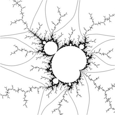
Figure 9 A copy of M witrnn M. The address of the copy is given by the arguments of the two external rays that+ land at the cusp, the root point of the copy. Here the arguments are and . Compare with figure 8. The rays are drawn to indicate where the “decorations” should be cut off in order to have the bare copy of M.

In the copy of M shown in figure 9, the “center” associated with c = 0 in M corresponds to a polynomial for which the critical point 0 is periodic of period 4, and for which a suitable restriction of the fourth iterate is quadratic-like from V₀ to its image W₀. Moreover, there is a neighborhood V₀ of c_O in the c-plane such that for any c in V₀ the restriction of f_c = to V₀ is a quadratic-like map from V₀ to its image W_c, and such that the map Ξ is a homeomorphism from to M.

The infinitely many copies of M that appear inside M may suggest that M has a self-similarity property. However, there is another phenomenon that pulls in the opposite direction. The c-values for which the critical point 0 is pre-periodic form a dense subset of ∂M. If is one of these special c-values, then there are two contexts in which one may look at magnifications of smaller and smaller neighborhoods of : the first is the Julia set J of the polynomial Q in neighborhoods of z = , and the second is the Mandelbrot set in neighborhoods of c =. It turns out that the pictures are asymptotically similar, which means that the greater the magnification, and the smaller the neighborhood, the more similar the two pictures become.

This is an extraordinary fact. Indeed, it may even seem to be impossible, since in any neighborhood of the Mandelbrot set contains infinitely many copies of itself, while the Julia set is known to contain no such copies. The explanation for the apparent paradox is that the copies of the Mandelbrot set get smaller very quickly as their distance to decreases. Hence, if one magnifies a small enough neighborhood, the copies that are there are practically invisible.

2.10 Newton’s Method Revisited

Let us return briefly to Newton’s method for polynomials. Consider any polynomial P of degree d ≥ 2 that has only simple roots. Then the Newton function N_p is a rational function of degree d, and each simple root of P is a super-attracting fixed point of N_p. For quadratic polynomials the number of roots of P coincides with the number of critical points of N_p (since 2d – 2 = 2 when d = 2). For polynomials of degree d > 2 there are more critical points than the roots can account for.

Cayley considered Newton’s method for quadratic polynomials with two distinct roots P(z) = (z–r₁) (z– r₂). He showed that the function μ(z) = (z – r₁) / (z–r₂), which maps the root r₁ onto 0 and the root r₂ onto ∞, provides a change of variables that turns N_P into the quadratic polynomial Q₀ on the Riemann sphere . When one translates the dynamics of Q₀ to the dynamics of Newton’s method one finds that the unit circle corresponds to the bisector of r_l and r₂ and that all points in the half-plane containing r_i = 1, 2, are therefore attracted to r_i under iteration by N_p.

Cayley announced that he would write about Newton’s iteration for cubic polynomials. However, it took about a hundred years before any such paper appeared. For a cubic polynomial P with three simple roots the Newton function N_P has three super-attracting fixed points, each of which gives rise to an attracting basin. The Julia set of N_p is the common boundary of these three basins, and is therefore a complicated fractal set. Moreover, N_P has an extra critical point since 2d–2 = 4 for d = 3. The extra critical point may be attracted to one of the roots under iteration, or it can have its own independent behavior. In order to catch the behavior of all cubic polynomials under Newton’s iteration (except the one with one root of multiplicity three) it is sufficient to consider the one-parameter family of polynomials P_λ (z) = (z - 1) (z – – λ) (z – + λ). The extra critical point for the corresponding Newton function N_λ then turns out to be at the origin. Suppose that we associate three colors, for instance red, blue, and green, with the three roots 1, + λ, – λ. We can then color the λ-plane, which is the parameter plane in this context, as follows. A parameter value λ is colored red, blue, or green if the critical point 0 is attracted under iteration by Nλ to the root of that color. If it is not attracted to any of the three roots, then we color with a fourth color, yellow, say. The universality of the Mandelbrot set is thereby demonstrated: in the λ-plane one can observe yellow copies of it, which one can explain by showing that families of suitably restricted iterates of N_λ are quadratic-like.

3 Concluding Remarks

We have illustrated several results in holomorphic dynamics through examples, including the transferring of definitions and results from the dynamical planes to the parameter plane. The structures of the filled Julia sets and the Mandelbrot set are partly understood through analysis of their complements, linked together via the Böttcher maps _c and Φ_M. The functions that are used for changing variables in J-stability and structural stability are examples of so-called quasiconformal mappings. This is a concept that was introduced into holomorphic dynamics in the early 1980s by Dennis Sullivan. They are indispensable for discussing change of complex structure, straightening, holomorphic motion, surgery, and many other phenomena. The interested reader is referred to the books listed below. The first two contain expository papers, the third is a graduate textbook, and the fourth is a collection of papers. They all contain many further references.

Acknowledgments. The computer drawings in this article were obtained from a program written by Christian Henriksen.

Further Reading

Devaney, R. L., and L. Keen, eds. 1989. Chaos and Fractals. The Mathematics Behind the Computer Graphics. Proceedings of Symposia in Applied Mathematics, volume 39. Providence, RI: American Mathematical Society.

——. 1994. Complex Dynamical Systems. The Mathematics Behind the Mandelbrot and Julia Sets. Proceedings of Symposia in Applied Mathematics, volume 49. Providence, RI: American Mathematical Society.

Lei, T., ed. 2000. The Mandelbrot Set, Theme and Variations. London Mathematical Society Lecture Note Series, volume 274. Cambridge: Cambridge University Press.

Milnor, J. 1999. Dynamics in One Complex Variable. Weisbaden: Vieweg.