---

III.91 Transforms

T. W. Körner

---

If we have a finite sequence a₀, a₁, . . . , a_n of real numbers (written briefly as a), then we can look at the polynomial

P_a(t)= a₀ + a₁t + ··· + a_ntⁿ.

Conversely, given a polynomial Q of degree m ≤ n, we can recover a unique sequence b₀, b₁, . . . , b_n such that

Q (t) = b₀ + b₁t + · · · + b_ntⁿ

by, for example, taking b_k = Q ^(k) (0) / k!.

We observe that if a₀, a₁, . . . ,a_n , and b₀, b₁, . . . , b_n are finite sequences, then

P_a(t)P_b(t) = p_a*b(t),

where a * b = c is a sequence c₀, c_l, . . . , c_2n given by

c_k = a₀b_k + a_lb_k-l + . . . + a_kb₀,

where we interpret a_i, and b_i as 0 if i > n. This sequence is called the convolution of the sequences a and b.

To see the kind of use that one can make of this observation, consider what happens when we throw two dice, the first of which has probability a_u of showing u and the second of which has probability b_υ of showing υ. The probability that their sum is k is given by the number c_k defined above. If we take both a_u and b_u to be the probability of throwing u with an ordinary fair die (so they are equal to if 1 ≤ u ≤ 6, and 0 otherwise), then

P_c(t) = P_a(t)P_b(t)

= ( (t + t² + ··· + t⁶))2.

This polynomial can be rewritten as

  (t(t + 1)(t⁴ + t² + 1))(t(t² + t + 1)(t³ + 1))

= (t(t + 1)(t² + t + 1))(t(t⁴ + t² + 1)(t³ + 1))

= P_A(t)P_B(t),

where A and B are two different sequences, given by A₁ = A₄ = , A₂ = A₃ = , and A_u = 0 otherwise, and B₁ = B₃ = B₄ = B₅ = B₆ = B₈ = , and B_υ = 0 otherwise. Thus, if we take two fair dice A and B and number A so that it has 2 on two faces, 3 on two faces, 1 on one face, and 4 on the remaining face, and we number B so that it has 1, 3, 4, 5, 6, and 8 on its faces, then the probability of throwing a sum k is the same as with an ordinary pair of dice. It is not hard to show, by considering the roots of the polynomial t + t² + · · · + t⁶, that this is the only nonstandard labeling of dice with strictly positive integers that has this property.

These general ideas are easily extended to infinite sequences. If a is the sequence a₀, a₁. . . , we can define an “infinite polynomial” (a) (t) to be . For the moment, we shall proceed formally, without worrying in what sense the sum exists. Observe that, much as before,

(a)(t)(b)(t) = ( (a * b))(t),

where the infinite sequence c = a * b is given by

C_k = a₀b_k + a₁b_{k -1} + . . . + a_kb₀.

(Again, we call this the convolution of a and b.)

There is a well-known problem in which we are asked how many ways there are of making change for r units of currency using notes of given denominations. (For example, we can ask how many ways there are of making $43 out of $1 and $5 bills.) If we can make r units in a_r ways using one set of denominations and b_r ways using a completely different set, then it is not hard to see that, if we are allowed to use both sets of denominations, we can make up k units in c_k ways, where c_k is again the number defined earlier.

Let us see how this applies in the simple case where a_r is the number of ways of making up r dollars using $1 bills and b_r is the number of ways of making up r dollars using $2 bills. We observe that

and so, using partial fractions,

Thus we can make change for r dollars in (r + 1) ways when r is odd and (r + 2) ways when r is even. In this simple case it is easy to obtain the result directly but the method indicated works automatically in all cases. (The calculations can be made easier if we allow ourselves to work with complex roots.)

We have produced a “generating function transform” or “-transform,” which takes a sequence a₀, a₁,. . . into a Taylor series . (These names are not standard: most mathematicians would simply talk about GENERATING FUNCTIONS [IV.18 §§2.4, 3].) The next two examples show how we can use -transforms to restate problems about sequences as problems about Taylor series. Consider first the problem of finding a sequence u_n such that u₀ = 0, u₁ = 1, and

u_{n + 2} - 5u_{n + 1} + 6u_n = 0

for all n ≥ 0. Observe that we must have

u_{n + 2}t^{n + 2} - 5u_{n + 1}t^{n + 2} + 6u_nt^{n + 2} = 0

for all n ≥ 0, so that summing over all n ≥ 0 yields ((u)(t)-u₁t-u₀)-5(t (u)(t)-u₀) + 6t² (u)(t) = 0. Recalling that u₀ = 0, u₁ = 1, and rearranging, we obtain

(6t² - 5t + 1)(u) (t) = t.

Thus, using partial fractions, we obtain

It follows that u_r = 3^r - 2^r

Next consider the rather trivial problem of finding a sequence u_n such that u₀ = 1 and

(n + 1) u_{n + 1} + u_n = 0

for all n ≥ 0. For every t we have

(n + 1)u_{n + 1} tⁿ + u_ntⁿ = 0

and so, summing over all n and assuming that the usual laws of differentiation apply to infinite sums, we obtain

(u)′(t) + (u)(t) = 0.

This differential equation gives (u) (t) = Ae^-t for some constant A. Setting t = 0, we obtain

1 = u₀ = (u) (0) = Ae⁰ = A.

Thus

so u_{r = (-1) ^r/r!.}

We can write down some of the correspondences between sequences and their -transforms:

It is also important that we can recover the sequence a from its -transform. One way of seeing this is to note that

We can use these rules, as in the examples above, to convert problems about sequences into problems about functions and vice versa. In textbooks and examinations, the effect of such a transformation is to make things simpler. In real life, it will usually convert your problem into a more complicated problem. However, occasionally you strike lucky and it is these occasions that make transforms such a valuable weapon in the mathematician’s armory.

Up to now we have handled -transforms formally. However, if we wish to use the methods of analysis, we need to know that converges, at least when |t| is small. Provided that the a_r do not increase too rapidly, this will always be the case. However, we run into difficulties when we try to extend our ideas to “two-sided sequences” (a_r), where r runs through all integers rather than just the nonnegative ones, and to the resulting sums . If |t| is small, then |t^r| is large when r is large and negative, while if |t| is large, then |t^r| is large when r is large and positive. In many cases, the best we can hope for is that might converge when t = -1 and t = 1. It is not very useful to talk about functions defined at only two points, but we save the situation by moving from to .

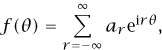
If we have a well-behaved sequence (a_r) of complex numbers where r runs through all integers, then we consider the sum a_rz^r, where the complex number z belongs to the unit circle (or, in other words, |z| = 1). Since any such z can be written

z = e^iθ = cos θ + i sin θ

with θ ∈ , it is more usual to talk about the 2π-periodic function We thus have the “Fourier series transform” (once again, the name is nonstandard) given by

The -transform takes a two-sided sequence a to a 2π-periodic complex-valued function f = a on the real line, but historically mathematicians have been more interested in reversing the process and obtaining a from f. If

then, arguing formally,

If we write

then we obtain the celebrated Fourier sum formula

DIRICHLET [VI.36] proved that this formula holds in its natural interpretation for reasonably well-behaved functions, but the question of the appropriate interpretation and proof for wider classes of functions took much longer to settle (see CARLESON’S THEOREM [V.5]). Aspects of the question are still open today.

It is worth noting that we can obtain qualitative information about a sequence from its -transform and vice versa without explicit calculation. For example, if a_rr^{m + 3} forms a bounded sequence, then the rules for term-by-term differentiation show that a is continuously m times differentiable, and if f is m times continuously differentiable, then repeated integration by parts shows that the numbers r^m (r) form a bounded sequence.

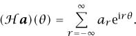
Suppose that f represents a signal fed into a “black box,” such as a telephone system, which gives rise to a resultant signal T f. Many important black boxes in physics and engineering have the “infinite linearity” property that

for all well-behaved function g_r and constants c_r. Many such systems also have the key property that

Te_k (θ) = γ_ke_k(θ)

for some constant γ_k, where we have written e_k(θ) for the quantity e-^ikθ. In other words, the functions e_k are EIGENFUNCTIONS [I.3 §4.3] for T. We can use the Fourier sum formula to obtain the formula

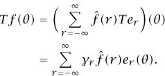
In this context, it makes sense to think of f as the weighted sum of simple signals e_k of frequency k.

Mathematicians are always interested to see what happens if sums are replaced by integrals. In this case we obtain the classical Fourier transform. If F is a reasonably well-behaved function F : → then we define its Fourier transform F by the formula

Much of the analysis that is typically taught in the first year or two of a university mathematics course was developed in the context of this transform and related topics. Using that analysis, it is not hard to obtain the correspondences

In this context we define the convolution of F and G by

There is an element of truth in the saying that the importance of the Fourier transform is that it converts convolution to multiplication and the importance of convolution is that it is the operation that is transformed to multiplication by the Fourier transform. Just as we can use the -transform to solve difference equations, we can use the -transform to solve important classes Of PARTIAL DIFFERENTIAL EQUATIONS [I.3 §5.4] that occur in physics and some parts of probability theory. For more on the Fourier transform, see [III.27].

By rescaling the Fourier sum formula (1), we obtain the formula

when |t| < πN. If we let N →. ∞, we obtain, more or less formally,

which translates to the marvelous formula

(F) (t) = 2πF (-t).

Like the Fourier sum formula, this Fourier inversion formula can be proved under a wide range of circumstances, though often at the price of reinterpreting the formula in novel ways.

Beautiful though the Fourier inversion formula is, it should be noted that, both in practice and in theory, we often need only the observation that F = G implies F = G. The uniqueness of the Fourier transform is often easier to prove and more convenient to use, and it holds over a wider range of conditions than the inversion formula. A similar observation holds for other transforms.

When we talked about the Fourier sums associated with 2π-periodic functions, we said that (r) measured the proportion of the signal f with frequency 2πr. In the same way, (F) (λ) gives a measure of the proportion of F composed of frequencies close to λ. There is a family of inequalities, known generically as Heisenberg uncertainty principles, which say, in effect, that if most of F is concentrated in a narrow band, then the signal F must be very spread out. This fact places strong restrictions on our ability to manipulate signals and occupies a central place in quantum theory.

At the beginning of this article we talked about transformations of sequences and saw that it was easier to handle one-sided sequences than two-sided sequences. In the same way, we can apply Fourier transforms to a wider range of functions F : → if we know that F (t) = 0 for t < 0. More specifically, if F is such a one- sided function, and if it does not grow too fast, then we can compute the Laplace transform

whenever x and y are real and x is sufficiently large. If we use the more natural notation

we see that F can be considered as a weighted average of HOLOMORPHIC [I.3 §5.6] (that is, complex differentiable) functions and this can be used to show that F is holomorphic. The Laplace transform shares many of the properties of the Fourier transform and we can use these, as well as the extensive collection of results on holomorphic functions, whenever we manipulate Laplace transforms. Many of the deepest results in number theory, such as the PRIME NUMBER THEOREM [V.26], are most easily obtained by clever uses of the Laplace transform.

The transforms we have discussed all belong to the same family, as is indicated by the fact that they all take convolution to multiplication. The general idea of a transform has been developed in several different directions, generally by concentrating on some aspects of the “classical transforms” and being prepared to lose others.

One of the most important of these new transforms is the Gelfand transform, which gives a concrete representation of the abstract commutative Banach algebras. It is discussed in OPERATOR ALGEBRAS [IV.15 §3.1]. Other integral transforms extend the integral definition of the Fourier transform by setting up a correspondence

F(t) F(s)K(λ -s) ds

or, more generally,

F(t) F(s)k(s,λ) ds.

Another interesting transform is the Radon or x- ray transform. We shall consider the three-dimensional case and talk very informally. Suppose we shine a beam of radiation through a body in direction u. Suppose also that f is a function defined on ³ that represents how much radiation is absorbed by different parts of the body. What we can measure is the amount of radiation absorbed along any given straight line. We might present some of this information in the form of a two-dimensional image, which could represent the amount absorbed by all lines in the direction u. In general, we can use f to define a new function

(F)(u, v) = f(tu + υ) dt,

which tells us how much radiation is absorbed along the line in direction u that goes through a vector υ perpendicular to u. The tomography problem deals with the recovery of f from f.

Because the idea of a transform has been developed in so many different directions, any attempt to give a general definition results in something too general to be useful. The most that we can say about the various transforms is that they present a more or less distant analogy to the classical Fourier transforms and that this analogy has been found useful by those who developed them. (See also THE FOURIER TRANSFORM [III.27], SPHERICAL HARMONICS [III.87], REPRESENTATION THEORY [IV.9 §3], and WAVELETS AND APPLICATIONS [VII.3].)