V.9 Ergodic Theorems

Vitaly Bergelson

Consider the sequence , where z is a complex number of modulus 1. While for z ≠ 1 our sequence is not convergent, it is not hard to see that, on average, it exhibits quite regular behavior. Indeed, using the formula for the sum of a geometric progression, and assuming that z ≠ 1, we have, for any N > M ≥ 0,

which implies that when N - M is large enough, the averages

are small. More formally, we have

This simple fact is a special, one-dimensional case of von Neumann’s ergodic theorem, which was the first mathematical statement to throw light on the so-called quasi-ergodic hypothesis in statistical mechanics and the kinetic theory of gases.

Von Neumann’s theorem concerns the average behavior of powers of UNITARY OPERATORS [III.50 §3.1] on HILBERT SPACES [III.37]. If U is such an operator defined on a Hilbert space , then we can associate with U the U-invariant subspace _inv that consists of all vectors f ∈ such that U f = f: that is, all vectors that are fixed by U. Let P be the ORTHOGONAL PROJECTION [III.50 §3.5] onto that subspace. Then von Neumann’s theorem asserts that, for every f ∈ ,

In other words, in a certain sense the averages

converge to the orthogonal projection P. (This is not actually the theorem as formulated by VON NEUMANN [VI.91], but it is simpler to explain. He proved an equivalent statement about a continuous family of unitary operators (U_T)_T∈.)

Before we discuss various applications and refinements of von Neumann’s theorem, let us briefly comment on its proof. Von Neumann’s original proof used sophisticated machinery such as the spectral theory of one-parameter groups of unitary operators, obtained by Marshall Stone. Over the years many alternative proofs were offered, the simplest being a “geometric” proof due to RIESZ [VI.74], which we will describe below. To give the rough idea of von Neumann’s proof it is convenient to use the fact (which follows from the SPECTRAL THEOREM [III.50 §3.4]) that any unitary operator U on a Hilbert space has a “functional model.” That is, we can realize the Hilbert space as a function space, consisting of all (equivalence classes of) square-integrable functions with respect to some finite MEASURE [III.5 5], in such away that U becomes a multiplication operator M (f) = f, where is a complex-valued measurable function that satisfies | (x) | = 1 for almost every x. It is not hard to see, after passing to such a functional model, that von Neumann’s theorem follows immediately from its one-dimensional case as expressed by formula (1). Note that in this case the orthogonal projection to the space of invariant elements takes a function f to the function g such that g(x) = f(x) if (x) = 1 and g(x) = 0 otherwise.

Riesz’s proof is based on the observation that the orthogonal complement of the subspace _inv of U-invariant vectors is spanned by the set of vectors of the form Ug - g. To see this, note first that if f ∈ _inv, then

〈f, Ug〉 = 〈U^–1 f, g) = 〈f, g〉,

from which it follows that 〈f, Ug – g〉 = 0 and thus that f is orthogonal to Ug – g. Conversely, if f ∉ _inv, then 〈f, Uf – f〉 = 〈f, Uf〉 – 〈f, f〉. This is less than 0, by the CAUCHY–SCHWARZ INEQUALITY [V.19] and the fact that ||Uf|| = ||f|| but Uf ≠ f. In particular, f is not orthogonal to Uf – f. Thus, _inv is the orthogonal complement of the (closed) subspace of generated by functions of the form Ug – g.

Now the conclusion of von Neumann’s theorem holds trivially if f ∈ _inv, since then P f = f and Uⁿf = f for every n. On the other hand, if f = Ug – g, then P f = 0. As for the averages, we know that Uⁿf = Uⁿ⁺¹g – Uⁿg, from which it follows that Uⁿf = U^Ng – U^Mg. Since ||U^Ng – U^Mg|| is at most 2||g|| for every M and N, we find that

has norm at most 2||g||/(N – M) and hence tends to 0. So the theorem is true in this case as well. It is straightforward to check that the set of functions for which the theorem holds is a closed linear subspace of , and therefore the theorem is proved.

The reason that von Neumann’s theorem and other similar results are relevant to physics is that it is often possible to represent the evolution of the parameters associated with a physical system by a subset X ⊂ ^d that has finite d-dimensional volume, together with a continuous family (T_τ)_τ∈ of volume-preserving transformations from X to X. With each such transformation T_τ one can associate the unitary map U_τ, defined on L² (X) (the Hilbert space of square-integrable functions on X) by the formula (U_τf)(x) = f(T_τx). The fact that these maps are unitary follows from the fact that the transformations T_τ preserve volume; also, it follows from the fact that the transformations T_τ depend continuously on τ that the maps U_τ do as well.

To simplify the discussion let us now “discretize” the situation. Instead of considering the continuous families (T_τ) and (U_τ) we shall fix a transformation T = T_τ0 (say, for τ₀ = 1) and let U be the corresponding unitary operator. Assume that our volume-preserving transformation T is ergodic, which means that there is no proper subset A ⊂ X of positive volume such that T(A) ⊂ A. This assumption can easily be shown to be equivalent to the fact that the only elements of L²(X) that satisfy Uf = f are the constant functions. It follows from von Neumann’s theorem that for any f ∈ L² (X) the averages

converge to a constant whose value is easy to find by performing term-by-term integration: it is equal to (∫ f dm)/vol(X). Since von Neumann’s theorem also tells us that lim_N–M→∞ A_N,M(f) is always a U-invariant function, we see that the assumption of ergodicity is a necessary and sufficient condition for the time average represented by _N–M→∞ A_N,M(f) to equal the space average, (∫ f dm)/vol(X).

It is also possible to use von Neumann’s theorem to strengthen a classical theorem of POINCARÉ [VI.61], called Poincaré’s recurrence theorem. This result states that if X is a set of finite volume, as above, and A is a subset of X with nonzero volume, then “almost all points of A return infinitely often to A.” In other words, if we set à to be the set of all points x ∈ A such that Tⁿx ∈ A for infinitely many n, then the measure of the set of points in A but not in à is 0. The main step in the proof of Poincaré’s theorem is to prove the same about the set A₁, which consists of all points x ∈ A such that Tⁿx ∈ A for some positive integer n. To see why this is true, let B be the set of all points in A but not in A₁. The sets B, T^–1B, T^–2B,. . . all have the same measure, since T is volume preserving. (T^–nB is defined to be the set of all x such that Tⁿx ∈ B.) Since X has finite volume, there must exist positive integers m and n such that the intersection of T^–mB and T–^(m+n) B has positive measure, and from this it follows that the measure of B ∩ T^–nB is also positive. But if x ∈ B then x ∉ A₁, so Tⁿx ∉ A and therefore Tⁿx ∉ B, so this is a contradiction.

Now let us apply the von Neumann ergodic theorem with f equal to the characteristic function of a set A (that is, f(x) = 1 when x ∈ A and f(x) = 0 otherwise) and U defined in terms of T as before. Suppose also that the set X has volume 1 and write μ for the measure on X. Then one can check that 〈f, Uⁿf〉 = μ(A ∩ T^–nA). It follows that

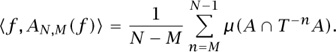
If we let N – M tend to infinity, then A_N,M f tends to a U-invariant function g. Since g is U-invariant, 〈f, g〉 = 〈Uⁿf, g〉 for every n, and therefore 〈f, g〉 = 〈A_N,M(f), g〉 for every N and M, and finally 〈f, g〉 = 〈g, g〉. By the Cauchy-Schwarz inequality, this is at least (∫ g(x) dμ)² = (∫ f (x) dμ)² = μ(A)². Therefore, we deduce that

If you choose two “random sets” of measure μ(A), then their intersection will typically be (μ(A))², so the inequality above is saying that the average intersection of A with T^–n A is at least as big as the “expected” intersection. This result, due to Khinchin, gives more precise information about the nature of Poincaré recurrence.

When a unitary operator is defined in terms of a measure-preserving transformation as above, it is natural to ask whether the averages converge not just in the sense of the L²-norm but also in the more classical sense of convergence almost everywhere. (For a related thought in a different context, see CARLESON’S THEOREM [V.5].) The answer is that they do, as was shown by BIRKHOFF [VI.78] soon after he learned of von Neumann’s theorem. He proved that for each integrable function f one could find a function f* such that f*(Tx) = f*(x) for almost every x, and such that

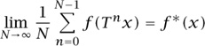
for almost every x. Suppose that the transformation T is ergodic, let A ∩ X be a set of positive measure, and let f (x) be the characteristic function of A. It follows from Birkhoff’s theorem that for almost every x ∈ X one has

Since the expression

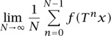
describes the frequency of visits of Tⁿx to the set A, we see that in an ergodic system the images x, Tx, T²x, . . . of a typical point x ∈ A visit A with a frequency that equals the proportion of the space occupied by A.

The ergodic theorems of von Neumann and Birkhoff have been generalized over the years in many different directions. These far-reaching extensions of ergodic theorems, and more generally the ergodic method, have found impressive applications in such diverse fields as statistical mechanics, number theory, probability theory, harmonic analysis, and combinatorics.

Further Reading

Furstenberg, H. 1981. Recurrence in Ergodic Theory and Combinatorial Number Theory. M. B. Porter Lectures. Princeton, NJ: Princeton University Press.

Krengel, U. 1985. Ergodic Theorems, with a supplement by A. Brunel. De Gruyter Studies in Mathematics, volume 6. Berlin: Walter de Gruyter.

Mackey, G. W. 1974. Ergodic theory and its significance for statistical mechanics and probability theory. Advances in Mathematics 12:178–268.

The Fermat–Euler Theorem

See MODULAR ARITHMETIC [III.58]