V.5 Carleson’s Theorem

Charles Fefferman

Carleson’s theorem asserts that the FOURIER SERIES [III.27] of a function f in L²[0, 2π] converges almost everywhere. To understand this statement and appreciate its significance, let us follow the history of the subject, starting in the early nineteenth century. FOURIER’S [VI.25] great idea was that “any” (complex-valued) function f on an interval such as [0, 2π] can be expanded in what we would now call a Fourier series,

for suitable Fourier coefficients a_n. Fourier obtained the formula for the coefficients a_n, and proved that (1) holds in interesting special cases.

The next major advance, due to DIRICHLET [VI.36], was a formula for the Nth partial sum S_Nf (θ), which is defined to be

Dirichlet realized that the precise meaning of (1) is that

Dirichlet used his formula for S_Nf to prove that under certain circumstances (3) does indeed hold. For example, if f is a continuous increasing function on [0, 2π], then it holds for every θ ∈ (0, 2π).

Decades later, DE LA VALLÉE POUSSIN [VI.67] discovered an example of a continuous function whose Fourier series diverges at a single point. More generally, given any countable set E ⊂ [0, 2π], there exists a continuous function f whose Fourier series diverges at every point of E, a result that appears to restrict quite considerably the circumstances under which Fourier’s original vision is valid.

The work of LEBESGUE [VI.72] led to fundamental progress in Fourier analysis and a significant change of viewpoint. We first sketch Lebesgue’s ideas and then trace their impact on Fourier analysis.

Lebesgue sought to define a notion of integration that could be applied to all but the most pathological nonnegative functions F on [0, 2π]. He began by defining the MEASURE [III.55] of a set E ⊂ [0, 2π]. Loosely speaking, the measure of E, written μ(E), is “what the set E would weigh” if the interval [0, 2π] were made of wire weighing one gram per centimeter. For instance, the measure of an interval (a, b) is equal to its length b – a. Certain sets E have measure zero, e.g., countable sets, or the CANTOR SET [III.17]; sets of measure zero are regarded as negligibly small.

Using his notion of measure, Lebesgue defined the Lebesgue integral F(θ) dθ for the “measurable” functions F ≥ 0 on [0, 2π]. All but the most pathological functions are measurable, but F(θ) dθ may be infinite if F is too big. For example, if F(θ) = 1 / θ for θ ∈ (0, 2π], then the integral of F is infinite

Finally, given any real number p ≥ 1, the Lebesgue space L^p[0, 2π] consists of all measurable functions f on [0, 2π] that are not too big, in the sense that |f (θ)|^p dθ is finite. (See FUNCTION SPACES [III.29] for a slight, technical correction to this definition.)

We now turn to the impact of Lebesgue’s theory on Fourier analysis. The Lebesgue space L²[0, 2π], which is also a HILBERT SPACE [III.37], plays a fundamental role. If f belongs to L²[0, 2π], then its Fourier coefficients a_n are such that

Conversely, any sequence of complex numbers a_n (-∞ < n < ∞) satisfying (4) arises as the sequence of Fourier coefficients of a function f in L² [0, 2π]. Moreover, the size of a function f and its Fourier coefficients a_n are related by the Plancherel formula:

Finally, the partial sums S_Nf (see (2)) converge to the function f in the L²-norm. In other words,

as N tends to infinity. This gives us a precise sense in which the function f is the sum of its Fourier series. Thus, we have justified Fourier’s formula (1) by reinterpreting it as the statement (5) rather than using the more obvious interpretation of (3).

However, it would still be nice to know to what extent the original, more straightforward interpretation can be justified. In 1906, Luzin conjectured that if f is any function in L² [0, π], then

for all θ outside a set of measure zero. When this holds, one says that the Fourier series of f converges almost everywhere. If Luzin’s conjecture were true, it would validate Fourier’s vision from the early nineteenth century.

For several decades it looked as though Luzin’s conjecture might well be false. KOLMOGOROV [VI.88] constructed a function f in L¹ [0, 2π] whose Fourier series converges nowhere. Also, a theorem of Kolmogorov, Seliverstov, and Plessner, which asserted that lim_{N → ∞} (S_N f (θ) / ) = 0 almost everywhere when f is in L² [0, 2π], withstood all attempts at improvement for over thirty years.

It therefore came as a big surprise when Lennart Carleson proved in 1966 that Luzin’s conjecture is true. The main point of Carleson’s proof is to control the Carleson maximal function

by proving that

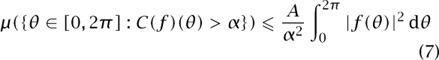
for all f in L²[0, 2π] and all α > 0, where A is a constant independent of f and α. It is not hard to show that (7) implies Luzin’s conjecture, but it is very hard to prove (7).

Shortly after Carleson’s work, Hunt proved the almost-everywhere convergence of Fourier series of functions in L^p [0, 2π] for any p > 1. Kolmogorov’s counterexample shows that the result fails for p = 1.

Fourier analysis has been immensely useful in mathematics and its applications. (For a fuller discussion of this, see THE FDURIER TRANSFORM [III.27] and HARMONIC ANALYSIS [IV.11].) The theorems of Carleson and Hunt provide the sharpest known answer to the basic question that started the subject.

Acknowledgments. This work was partially supported by NSF grant #DMS-0245242.

Cauchy’s Theorem

See SOME FUNDAMENTAL MATHEMATICAL DEFINITIONS [I.3 § 5.6]