---

IV.25 Probabilistic Models of Critical Phenomena

Gordon Slade

---

1 Critical Phenomena

1.1 Examples

A population can explode if its birth rate exceeds its death rate, but otherwise it becomes extinct. The nature of the population’s evolution depends critically on which way the balance tips between adding new members and losing old ones.

A porous rock with randomly arranged microscopic pores has water spilled on top. If there are few pores, the water will not percolate through the rock, but if there are many pores, it will. Surprisingly, there is a critical degree of porosity that exactly separates these behaviors. If the rock’s porosity is below the critical value, then water cannot flow completely through the rock, but if its porosity exceeds the critical value, even slightly, then water will percolate all the way through.

A block of iron placed in a magnetic field will become magnetized. If the magnetic field is extinguished, then the iron will remain magnetized if the temperature is below the Curie temperature 770 °C (1418 °F), but not if the temperature is above this critical value. It is striking that there is a specific temperature above which the magnetization of the iron does not merely remain small, but actually vanishes.

The above are three examples of critical phenomena. In each example, global properties of the system change abruptly as a relevant parameter (fertility, degree of porosity, or temperature) is varied through a critical value. For parameter values just below the critical value, the overall organization of the system is quite different from how it is for values just above. The sharpness of the transition is remarkable. How does it occur so suddenly?

1.2 Theory

The mathematical theory of critical phenomena is currently undergoing intense development. Intertwined with the science of phase transitions, it draws on ideas from probability theory and statistical physics. The theory is inherently probabilistic: each possible configuration of the system (e.g., a particular arrangement of pores in a rock, or of the magnetic states of the individual atoms in a block of iron) is assigned a probability, and the typical behavior of this ensemble of random configurations is analyzed as a function of parameters of the system (e.g., porosity or temperature).

The theory of critical phenomena is now guided to a large degree by a profound insight from physics known as universality, which, at present, is more of a philosophy than a mathematical theorem. The notion of universality refers to the fact that many essential features of the transition at a critical point depend on relatively few attributes of the system under consideration. In particular, simple mathematical models can capture some of the qualitative and quantitative features of critical behavior in real physical systems even if the models dramatically oversimplify the local interactions present in the real systems. This observation has helped to focus attention on particular mathematical models, among both physicists and mathematicians.

This essay discusses several models of critical phenomena that have attracted much attention from mathematicians, namely branching processes, the model of random networks known as the random graph, the percolation model, the Ising model of ferromagnetism, and the random cluster model. As well as having applications, these models are mathematically fascinating. Deep theorems have been proved, but many problems of central importance remain unsolved and tantalizing conjectures abound.

2 Branching Processes

Branching processes provide perhaps the simplest example of a phase transition. They occur naturally as a model of the random evolution of a population that changes in time as a result of births and deaths. The simplest branching process is defined as follows.

Consider an organism that lives for a unit time and that reproduces immediately before death. The organism has two potential offspring, which we can regard as the “left” offspring and the “right” offspring. At the moment of reproduction, the organism has either no offspring, a left but no right offspring, a right but no left offspring, or both a left and a right offspring. Assume that each of the potential offspring has a probability p of being born and that these two births occur independently. Here, the number p, which lies between 0 and 1, is a measure of the population’s fecundity. Suppose that we start with a single organism at time zero, and that each descendant of this organism reproduces independently in the above manner.

A possible family tree is depicted in figure 1, showing all births that occurred. In this family tree, ten offspring were produced in all, but twelve potential offspring were not born, so the probability of this particular tree occurring is p¹⁰(1 - p)¹².

If p = 0, then no offspring are born, and the family tree always consists of the original organism only. If p = 1, then all possible offspring are born, the family tree is the infinite binary tree, and the population always survives forever. For intermediate values of p, the population may or may not survive forever: let θ(p) denote the survival probability, that is, the probability that the branching process survives forever when the fecundity is set at p. How does θ(p) interpolate between the two extremes θ(0) = 0 and θ(1) = 1?

Figure 1 A possible family tree, with probability p¹⁰(1 - p)¹².

2.1 The Critical Point

Since an organism has each of two potential offspring independently with probability p, it has, on average, 2p offspring. It is natural to suppose that survival for all time will not occur if p < , since then each organism, on average, produces less than 1 offspring. On the other hand, if p > , then, on average, organisms more than replace themselves, and it is plausible that a population explosion can lead to survival for all time.

Branching processes have a recursive nature, not present in other models, that facilitates explicit computation. Exploiting this, it is possible to show that the survival probability is given by

The value p = p_c = is a critical value, at which the graph of θ(p) has a kink (see figure 2). The interval p < p_c is referred to as subcritical, whereas p > p_c is supercritical.

Rather than asking for the probability θ(p) that the initial organism has infinitely many descendants, one could ask for the probability P_k(p) that the number of descendants is at least k. If there are at least k + 1 descendants, then there are certainly at least k, so P_k(p) decreases as k increases. In the limit as k increases to infinity, P_k(p) decreases to θ(p). In particular, when p > p_c, P_k(p) approaches a positive limit as k approaches infinity, whereas P_k(p) goes to zero when p ≤ p_c. When p is strictly less than p_c, it can be shown that P_k(p) goes to zero exponentially rapidly, but at the critical value itself we have

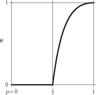
Figure 2 The survival probability θ versus p.

The symbol “~” denotes asymptotic behavior, and means that the ratio of the left- and right-hand sides in the above formula goes to 1 as k goes to infinity. In other words, P_k(p_c) behaves essentially like 2/ when k is large.

There is a pronounced difference between the exponential decay of P_k(p_c) for p < p_c and the square-root decay at p_c. When p = , family trees larger than 100 are sufficiently rare that in practical terms they do not occur: the probability is less than 10^-14. However, when p = p_c, roughly one in every ten trees will have size at least 100, and roughly one in a thousand will have size at least 1 000 000. At the critical value, the process is poised between extinction and survival.

Another important attribute of the branching process is the average size of a family tree, denoted (p). A calculation shows that

In particular, the average family size becomes infinite at the same critical value p_c = above which the probability of an infinite family ceases to be zero. The graph of is shown in figure 3. At p = p_c, it may seem at first sight contradictory that family trees are always finite (since θ(p_c) = 0) and yet the average family size is infinite (since (p_c) = ∞). However, there is no inconsistency, and this combination, which occurs only at the critical point, reflects the slowness of the square-root decay of P_k(p_c).

Figure 3 The average family size versus p.

2.2 Critical Exponents and Universality

Some aspects of the above discussion are specific to twofold branching, and will change for a branching process with higher-order branching. For example, if each organism has not two but m potential offspring, again independently with probability p, then the average number of offspring per organism is mp and the critical probability p_c changes to 1/m. Also, the formulas written above for the survival probability, for the probability of at least k descendants, and for the average family size must all be modified and will involve the parameter m.

However, the way that θ(p) goes to zero at the critical point, the way that P_k(p_c) goes to zero as k goes to infinity, and the way that (p) diverges to infinity as p approaches the critical point p_c will all be governed by exponents that are independent of m. To be more specific, they behave in the following manner:

Here, the numbers C1, C2, and C3 are constants that depend on m. By contrast, the exponents β, δ, and γ take on the same values for every m ≥ 2. Indeed, those values are β = 1, δ = 2, and γ = 1. They are called critical exponents, and they are universal in the sense that they do not depend on the precise form of the law that governs how the individual organisms reproduce. Related exponents will appear below in other models.

3 Random Graphs

An active research field in discrete mathematics with many applications is the study of objects known as GRAPHS [III.34]. These are used to model systems such as the Internet, the World Wide Web, and highway networks. Mathematically, a graph is a collection of vertices (which might represent computers, Web pages, or cities) joined in pairs by edges (physical connections between computers, hyperlinks between Web pages, highways). Graphs are also called networks, vertices are also called nodes or sites, and edges are also called links or bonds.

3.1 The Basic Model of a Random Graph

A major subarea of graph theory, initiated by Erdős and Rényi in 1960, concerns the properties that a graph typically has when it has been generated randomly. A natural way to do this is to take n vertices and for each pair to decide randomly (by the toss of a coin, say) whether it should be linked by an edge. More generally, one can choose a number p between 0 and 1 and let p be the probability that any given pair is linked. (This would correspond to using a biased coin to make the decisions.) The properties of random graphs come into their own when n is large, and of particular interest is the fact that there is a phase transition.

3.2 The Phase Transition

If x and y are vertices in a graph, then a path from x to y is a sequence of vertices that starts with x and ends with y in such a way that neighboring terms of the sequence are joined by edges. (If the vertices are represented by points and the edges by lines, then a path is a way of getting from x to y by traveling along the lines.) If x and y are joined by a path, then they are said to be connected. A component, or connected cluster, in a graph is what you obtain if you take a vertex together with all the other vertices that are connected to it.

Any graph decomposes naturally into its connected clusters. These will, in general, have different sizes (as measured by the number of vertices), and given a graph it is interesting to know the size of its largest cluster, which we shall denote by N. If we are considering a random graph with n vertices, then the value of N will depend on the multitude of random choices made when the graph was generated, and thus N is itself a random variable. The possible values of N are everything from 1, the value it takes when no edges are present and every cluster consists of a single vertex, to n, when there is just one connected cluster consisting of all the vertices. In particular, N = 1 when p = 0, and N = n when p = 1. At a certain point between these extremes, N undergoes a dramatic jump.

It is possible to guess where the jump might take place, by considering the degree of a typical vertex x. This means the number of neighbors of x, that is, other vertices that are directly linked to x by a single edge. Each vertex has n - 1 potential neighbors, and for each one the probability that it is an actual neighbor is p, so the expected degree of any given vertex is p (n - 1). When p is less than 1/(n - 1), each vertex has, on average, less than one neighbor, whereas when p exceeds 1/(n - 1), it has, again on average, more than one. This suggests that p_c = 1/(n - 1) will be a critical value, with N being small when p is below p_c, and large when p is above p_c.

This is indeed the case. If we set p_c = 1/(n - 1) and write p = p_c(1 + ε), with ε a fixed number between – 1 and +1, then ε = p(n - 1) – 1. Since p(n - 1) is the average degree of each vertex, ε is a measure of how much the average degree differs from 1. Erdős and Rényi showed that, in an appropriate sense, as n goes to infinity,

The A in the above formula is not a constant but a certain random variable that is independent of n (the distribution of which we have not specified here). When ε = 0 and n is large, the formula will tell us, for any a < b, the approximate probability that N lies between an^2/3 and bn^2/3. To put it another way, A is the limiting distribution of the quantity n^-2/3N when ε = 0.

There is a marked difference between the behavior of the functions log n, n^2/3, and n, for large n. The small clusters present for p < p_c correspond to what is called a subcritical phase, whereas in the so-called supercritical phase, where p > p_c, there is a “giant cluster” whose size is of the same order of magnitude as the entire graph (see figure 4).

It is interesting to consider the “evolution” of the random graph, as p is increased from subcritical to supercritical values. (Here one can imagine more and more edges being randomly added to the graph.) A remarkable coalescence occurs, in which many smaller clusters rapidly merge into a giant cluster whose size is proportional to the size of the entire system. The coalescence is thorough, in the sense that in the supercritical phase the giant cluster dominates everything: indeed, the second-largest cluster is known to have asymptotic size only 2ε^–2 log n, which makes it far smaller than the giant cluster.

p = p_c = 0.0012

p = p_c = 0.0020

Figure 4 The largest cluster (black) and second largest cluster (dots) in random graphs with 625 vertices. These clusters have sizes (a) 17 and 11 and (b) 284 and 16. The hundreds of edges in the graphs are not clearly shown.

3.3 Cluster Size

For branching processes, we defined the quantity (p) to be the average size of the family tree spawned by an individual when the probability of each potential offspring being born was p. By analogy, for the random graph it is natural to take an arbitrary vertex v and define (p) to be the average size of the connected cluster containing v. Since all the vertices play identical roles, (p) is independent of the particular choice of v. If we fix a value of ε, set p = p_c(1 + ε), and let n tend to infinity, it turns out that the behavior of (p) is described by the formula

where c is a constant. Thus the expected cluster size is independent of n when ε < 0, grows like n^1/3 when p = p_c, and is much larger—indeed, of the same order of magnitude n as the entire system—when ε > 0.

To continue the analogy with branching processes, let P_k(p) denote the probability that the cluster containing the arbitrary vertex v consists of at least k vertices. Again this does not depend on the particular choice of v. In the subcritical phase, when p = p_c (1 + ε) for some fixed negative value of ε, the probability P_k(p) is essentially independent of n and is exponentially small in k. Thus, large clusters are extremely rare. However, at the critical point p = p_c, P_k(p) decays like a multiple of 1/ (for an appropriate range of k). This much slower square-root decay is similar to what happens for branching processes.

3.4 Other Thresholds

It is not only the largest cluster size that jumps. Another quantity that does so is the probability that a random graph is connected, meaning that there is a single connected cluster that contains all the n vertices. For what values of the edge-probability p is this likely? It is known that the property of being connected has a sharp threshold, at p_conn = (1/n) log n, in the following sense. If p = p_conn(1 + ε) for some fixed negative ε, then the probability that the graph is connected approaches 0 as n → ∞. If on the other hand ε is positive, then the probability approaches 1. Roughly speaking, if you add edges randomly, then the graph suddenly changes from being almost certainly not connected to almost certainly connected as the proportion of edges present moves from just below p_conn to just above it.

There is a wide class of properties with thresholds of this sort. Other examples include the absence of any isolated vertex (a vertex with no incident edge), and the presence of a Hamiltonian cycle (a closed loop that visits every vertex exactly once). Below the threshold, the random graph almost certainly does not have the property, whereas above the threshold it almost certainly does. The transition occurs abruptly.

Figure 5 Bond-percolation configurations on a 14 × 14 piece of the square lattice ² for p = 0.25, p = 0.45, p = 0.55, p = 0.75. The critical value is p_c = .

4 Percolation

The percolation model was introduced by Broadbent and Hammersley in 1957 as a model of fluid flow in a porous medium. The medium contains a network of randomly arranged microscopic pores through which fluid can flow. A d-dimensional medium can be modeled with the help of the infinite d-dimensional lattice ^d, which consists of all points x of the form (x₁, . . ., x_d), where each x_i is an integer. This set can be made into a graph in a natural way if we join each point to the 2d points that differ from it by ±1 in one coordinate and are the same in the others. (So, for example, in ² the neighbors of (2, 3) are the four points (1, 3), (3, 3), (2, 2), and (2, 4).) One thinks of the edges as representing all pores potentially present in the medium.

To model the medium itself, one first chooses a porosity parameter p, which is a number between 0 and 1. Each edge (or bond) of the above graph is then retained with probability p and deleted with probability 1 - p, with all choices independent. The retained edges are referred to as “occupied” and the deleted ones as “vacant.” The result is a random subgraph of ^d whose edges are the occupied bonds. These model the pores actually present in a macroscopic chunk of the medium.

For fluid to flow through the medium there must be a set of pores connected together on a macroscopic scale. This idea is captured in the model by the existence of an infinite cluster in the random subgraph, that is, a collection of infinitely many points all connected to one another. The basic question is whether or not an infinite cluster exists. If it does, then fluid can flow through the medium on a macroscopic scale, and otherwise it cannot. Thus, when an infinite cluster exists, it is said that “percolation occurs.”

Percolation on the square lattice ² is depicted in figure 5. Percolation in a three-dimensional physical medium is modeled using ³. It is instructive, and mathematically interesting, to think how the model’s behavior might change as the dimension d is varied.

For d = 1, percolation will not occur unless p = 1. The simple observation that leads to this conclusion is the following. Given any particular sequence of m consecutive edges, the probability that they are all occupied is p^m, and if p < 1, then this goes to zero as m goes to infinity. The situation is quite different for d ≥ 2.

4.1 The Phase Transition

For d ≥ 2, there is a phase transition. Let θ(p) denote the probability that any given vertex of ^d is in an infinite connected cluster. (This probability does not depend on the choice of vertex.) It is known that for d ≥ 2 there is a critical value p_c, depending on d, such that θ(p) is zero if p < p_c and positive if p > p_c. The exact value of p_c is not known in general, but a special symmetry of the square lattice allows for a proof that p_c = when d = 2.

Using the fact that θ(p) is the probability that any particular vertex lies in an infinite cluster, it can be shown that when θ(p) > 0 there must be an infinite connected cluster somewhere in ^d, while when θ(p) = 0 there will not be one. Thus, percolation occurs when p > p_c but not when p < p_c, and the system’s behavior changes abruptly at the critical value. A deeper argument shows that when p > p_c there must be exactly one infinite cluster; infinite clusters cannot coexist on ^d. This is analogous to the situation in the random graph, where one giant cluster dominates when p is above the critical value.

Let (p) denote the average size of the connected cluster containing a given vertex. Certainly (p) is infinite for p > p_c, since then there is a positive probability that the given vertex is in an infinite cluster. It is conceivable that (p) could be infinite also for some values of p less than p_c, since infinite expectation is in principle compatible with θ(p) = 0. However, it is a nontrivial and important theorem of the subject that this is not the case: (p) is finite for all p < p_c and diverges to infinity as p approaches p_c from below.

Qualitatively, the graphs of θ and have the appearance depicted for the branching process in figures 2 and 3, although the critical value will be less than for d ≥ 3. There is, however, a caveat. It has been proved that θ is continuous in p except possibly at p_c, and right-continuous for all p. It is widely believed that θ is equal to zero at the critical point, so that θ is continuous for all p and percolation does not occur at the critical point. But proofs that θ(p_c) = 0 are currently known only for d = 2, for d ≥ 19, and for certain related models when d > 6. The lack of a general proof is all the more intriguing since it has been proved for all d ≥ 2 that there is zero probability of an infinite cluster in any half-space when p = p_c. This still allows for an infinite cluster with an unnatural spiral behavior, for example, though it is believed that this does not occur.

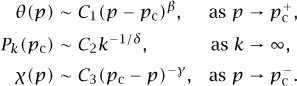
4.2 Critical Exponents

Assuming that θ(p) does in fact approach zero as p is decreased to p_c, it is natural to ask in what manner this occurs. Similarly, we can ask in what manner (p) diverges as p increases to p_c. Deep arguments of theoretical physics, and substantial numerical experimentation, have led to the prediction that this, as well as other, behavior is described by certain powers known as critical exponents. In particular, it is predicted that there are asymptotic formulas

The critical exponents here are the powers β and γ, which depend, in general, on the dimension d. (The letter C is used to denote a constant whose precise value is inessential and may change from line to line.)

When p is less than p_c, large clusters have exponentially small probabilities. For example, in this case the probability P_k(p) that the size of the connected cluster containing any given vertex exceeds k is known to decay exponentially as k → ∞. At the critical point, this exponential decay is predicted to be replaced by a power-law decay involving a number δ, which is another critical exponent:

P_k(p_c) ~ Ck^-1/δ as k → ∞.

Also, for p < p_c, the probability τ_p(x,y) that two vertices x and y are in the same connected cluster decays exponentially like e^{-|x – y|/ξ(p)} as the separation between x and y is increased. The number ξ(p) is called the correlation length. (Roughly speaking, τ_p(x,y) starts to become small when the distance between x and y exceeds ξ(p).) The correlation length is known to diverge as p increases to p_c, and the predicted form of this divergence is

where ν is a further critical exponent. As before, the decay at the critical point is no longer exponential. It is predicted that τ_pc(x,y) decays instead via a power law, traditionally written in the form

for yet another critical exponent η.

The critical exponents describe large-scale aspects of the phase transition and thus provide information relevant to the macroscopic scale of the physical medium. However, in most cases they have not been rigorously proved to exist. To do so, and to establish their values, is a major open problem in mathematics, one of central importance for percolation theory.

In view of this, it is important to be aware of a prediction from theoretical physics that the exponents are not independent, but are related to each other by what are called scaling relations. Three scaling relations are

γ = (2 – η)ν, γ + 2β = β(δ + 1), dν = γ + 2β.

4.3 Universality

Since the critical exponents describe large-scale behavior, it seems plausible that they might depend only weakly on changes in the fine structure of the model. In fact, it is a further prediction of theoretical physics, one that has been verified by numerical experiments, that the critical exponents are universal, in the sense that they depend on the spatial dimension d but on little else.

For example, if the two-dimensional lattice ² is replaced by another two-dimensional lattice, such as the triangular or the hexagonal lattice, then the values of the critical exponents are believed not to change. Another modification, for general d ≥ 2, is to replace the standard percolation model with the so-called spread-out model. In the spread-out model, the edge set of ^d is enriched so that now two vertices are joined whenever they are separated by a distance of L or less, where L ≥ 1 is a fixed finite parameter, usually taken to be large. Universality suggests that the critical exponents for percolation in the spread-out model do not depend on the parameter L.

The discussion so far falls within the general framework of bond percolation, in which it is bonds (edges) that are randomly occupied or vacant. A much-studied variant is site percolation, where now it is vertices, or “sites,” that are independently “occupied” with probability p and “vacant” with probability 1 - p. The connected cluster of a vertex x consists of the vertex x itself together with those occupied vertices that can be reached by a path that starts at x, travels along edges in the graph, and visits only occupied vertices. For d ≥ 2, site percolation also experiences a phase transition. Although the critical value for site percolation is different from the critical value for bond percolation, it is a prediction of universality that site and bond percolation on ^d have the same critical exponents.

These predictions are mathematically very intriguing: the large-scale properties of the phase transition described by critical exponents appear to be insensitive to the fine details of the model, in contrast to features like the value of critical probability p_c, which depends heavily on such details.

At the time of writing, the critical exponents have been proved to exist, and their values rigorously computed, only for certain percolation models in dimensions d = 2 and d > 6, while a general mathematical understanding of universality remains an elusive goal.

4.4 Percolation in Dimensions d > 6

Using a method known as the lace expansion, it has been proved that the critical exponents exist, with values

β = 1, γ = 1, δ = 2, ν = , η = 0,

for percolation in the spread-out model when d > 6 and L is large enough. The proof makes use of the fact that vertices in the spread-out model have many neighbors. For the more conventional nearest-neighbor model, where bonds have length 1 and there are fewer neighbors per vertex, results of this type have also been obtained, but only in dimensions d ≥ 19.

The above values of β, γ, and δ are the same as those observed previously for branching processes. A branching process can be regarded as percolation on an infinite tree rather than on ^d, and thus percolation in dimensions d > 6 behaves like percolation on a tree. This is an extreme example of universality, in which the critical exponents are also independent of the dimension, at least when d > 6.

If the above values for the exponents are substituted into the scaling relation dν = γ + 2β, the result is d = 6. Thus, the scaling relation (called a hyperscaling relation because of the presence of the dimension d in the equation) is false for d > 6. However, this particular relation is predicted to apply only in dimensions d ≥ 6. In lower dimensions, the nature of the phase transition is affected by the manner in which critical clusters fit into space, and the nature of the fit is partly described by the hyperscaling relation, in which d appears explicitly.

The critical exponents are predicted to take on different values below d = 6. Recent advances have shed much light on the situation for d = 2, as we shall see in the next section.

4.5 Percolation in Dimension 2

4.5.1 Critical Exponents and Schramm–Loewner Evolution

For site percolation on the two-dimensional triangular lattice it has been shown, in a major recent achievement, that the critical exponents exist and take the remarkable values

The scaling relations play an important role in the proof, but an essential additional step requires understanding of a concept known as the scaling limit.

To get some idea of what this is, let us look at the so-called exploration process, which is depicted in figure 6. In figure 6, hexagons represent vertices of the triangular lattice. Hexagons in the bottom row have been colored gray on the left half and white on the right half. The other hexagons have been chosen to be gray or white independently with probability , which is the critical probability for site percolation on the triangular lattice. It is not hard to show that there is a path, also illustrated in figure 6, which starts at the bottom and all along its length is gray to the left and white to the right. The exploration process is this random path, which can be thought of as the gray/white interface. The boundary conditions at the bottom force it to be infinite

The exploration process provides information about the boundaries separating large critical clusters of different color, and from this it is possible to extract information about critical exponents. It is the macroscopic large-scale structure that is essential, so interest is focused on the exploration process in the limit as the spacing between vertices of the triangular lattice goes to zero. In other words, what does the curve in figure 6 typically look like in the limit as the size of the hexagons shrinks to zero? It is now known that this limit is described by a newly discovered STOCHASTIC PROCESS [IV.24 §1] called the Schramm–Loewner evolution (SLE) with parameter six, or SLE6 for short. The SLE processes were introduced by Schramm in 2000, and have become a topic of intense current research activity.

Figure 6 The exploration process.

This is a major step forward in the understanding of two-dimensional site percolation on the triangular lattice, but much remains to be done. In particular, it is still an unsolved problem to prove universality. There is currently no proof that critical exponents exist for bond percolation on the square lattice ², although universality predicts that the critical exponents for the square lattice should also take on the interesting values listed above.

4.5.2 Crossing Probabilities

In order to understand two-dimensional percolation, it is very helpful to understand the probability that there will be a path from one side of a region of the plane to another, especially when the parameter p takes its critical value p_c.

To make this idea precise, fix a simply connected region in the plane (i.e., a region with no holes), and fix two arcs on the boundary of the region. The crossing probability (which depends on p) is the probability that there is an occupied path inside the region that joins one arc to the other, or more accurately the limit of this probability as the lattice spacing between vertices is reduced to zero. For p < p_c, clusters with diameter much larger than the correlation length ξ(p) (measured by the number of steps in the lattice) are extremely rare. However, to cross the region, a cluster needs to be larger and larger as the lattice spacing goes to zero. It follows that the crossing probability is 0. When p > p_c, there is exactly one infinite cluster, from which it can be deduced that if the lattice spacing is very small, then with very high probability there will be a crossing of the region. In the limit, the crossing probability is 1. What if p = p_c? There are three remarkable predictions for critical crossing probabilities.

Figure 7 The two regions are related by a conformal transformation, depicted in the upper figures. In the lower figures, the limiting critical crossing probabilities are identical.

The first prediction is that critical crossing probabilities are universal, which is to say that they are the same for all finite-range two-dimensional bond- or site-percolation models. (As always, we are talking about the limiting probabilities as the lattice spacing goes to zero.)

The second prediction is that the critical crossing probabilities are conformally invariant. A conformal transformation is a transformation that locally preserves angles, as shown in V.34] states that any two simply connected regions that are not the entire plane are related by a conformal transformation. The statement that the critical crossing probability is conformally invariant means that if one region with two specified boundary arcs is mapped to another region by a conformal transformation, then the critical crossing probability between the images of the arcs in the new region is identical to the crossing probability of the original region. (Note that the underlying lattice is not transformed; this is what makes the prediction so striking.)

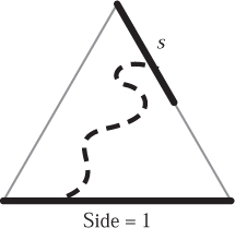
Figure 8 For the equilateral triangle of unit side length, Cardy’s formula asserts that the limiting critical crossing probability shown is simply the length s.

The third prediction is Cardy’s explicit formula for critical crossing probabilities. Assuming conformal invariance, it is only necessary to give the formula for one region. For an equilateral triangle, Cardy’s formula is particularly simple (see figure 8).

In 2001, in a celebrated achievement, Smirnov studied critical crossing probabilities for site percolation on the triangular lattice. Using the special symmetries of this particular model, Smirnov proved that the limiting critical crossing probabilities exist, that they are conformally invariant, and that they obey Cardy’s formula. To prove universality of the crossing probabilities remains a tantalizing open problem.

5 The Ising Model

In 1925, Ising published an analysis of a mathematical model of ferromagnetism which now bears his name (although it was in fact Ising’s doctoral supervisor Lenz who first defined the model). The Ising model occupies a central position in theoretical physics, and is of considerable mathematical interest.

5.1 Spins, Energy, and Temperature

In the Ising model, a block of iron is regarded as a collection of atoms whose positions are fixed in a crystalline lattice. Each atom has a magnetic “spin,” which is assumed for simplicity to point upward or downward. Each possible configuration of spins has an associated energy, and the greater this energy is, the less likely the configuration is to occur.

On the whole, atoms like to have the same spin as their immediate neighbors, and the energy reflects this: it increases according to the number of pairs of neighboring spins that are not aligned with each other. If there is an external magnetic field, also assumed to be directed up or down, then there is an additional contribution: atoms like to be aligned with the external field, and the energy is greater the more spins there are that are not aligned with it. Since configurations with higher energy are less likely, spins have a general tendency to align with each other, and also to align with the direction of the external magnetic field. When a larger fraction of spins points up than down, the iron is said to have a positive magnetization.

Although energy considerations favor configurations with many aligned spins, there is a competing effect. As the temperature increases, there are more random thermal fluctuations of the spins, and these diminish the amount of alignment. Whenever there is an external magnetic field, the energy effects predominate and there is at least some magnetization, however high the temperature. However, when the external field is turned off, the magnetization persists only if the temperature is below a certain critical temperature. Above this temperature, the iron will lose its magnetization.

The Ising model is a mathematical model that captures the above picture. The crystalline lattice is modeled by the lattice ^d. Vertices of ^d represent atomic positions, and the atomic spin at a vertex x is simply modeled by one of the two numbers +1 (representing spin up) or -1 (representing spin down). The particular number chosen at x is denoted σ_x, and a collection of choices, one for each x in the lattice, is called a configuration of the Ising model. The configuration as a whole is denoted simply as σ. (Formally, a configuration σ is a function from the lattice to the set {-1, 1}.)

Each configuration σ comes with an associated energy, defined as follows. If there is no external field, the energy of σ consists of the sum, taken over all pairs of neighboring vertices 〈x,y〉, of the quantity -σ_xσ_y. This quantity is -1 if σ_x = σ_y, and is +1 otherwise, so the energy is indeed larger the more nonaligned pairs there are. If there is a nonzero external field, modeled by a real number h, then the energy receives an additional contribution -hσ_x, which is larger the more spins there are with a different sign from that of h. Thus, in total, the energy E(σ) of a spin configuration σ is defined by

where the first sum is over neighboring pairs of vertices, the second sum is over vertices, and h is a real number that may be positive, negative, or zero.

The sums defining E(σ) actually make sense only when there are finitely many vertices, but one wishes to study the infinite lattice ^d. This problem is handled by restricting ^d to a large finite subset and later taking an appropriate limit, the so-called thermodynamic limit. This is a well-understood process that will not be described here.

Two features remain to be modeled, namely, the manner in which lower-energy configurations are “preferred,” and the manner in which thermal fluctuations can lessen this preference. Both features are handled simultaneously, as follows. We wish to assign to each configuration a probability that decreases as its energy increases. According to the foundations of statistical mechanics, the right way to do this is to make the probability proportional to the so-called Boltzmann factor e^-E(σ)/T, where T is a nonnegative parameter that represents the temperature. Thus, the probability is

where the normalization constant, or partition function, Z, is defined by

where the sum is taken over all possible configurations σ (again it is necessary to work first in a finite subset of ^d to make this precise). The reason for this choice of Z is that once we divide by it then we have ensured that the probabilities of the configurations add up to one, as they must. With this definition, the desired preference for low energy is achieved, since the probability of a given configuration is smaller when the energy of the configuration is larger. As for the effect of the temperature, note that when T is very large, all the numbers e^-E(σ)/T are close to 1, so all probabilities are roughly equal. In general, as the temperature increases the probabilities of the various configurations become more similar, and this models the effect of random thermal fluctuations.

There is more to the story than energy, however. The Boltzmann factor makes any individual low-energy configuration much more likely than any individual high- energy configuration. However, the low-energy configurations have a high degree of alignment, so there are far fewer of them than there are of the more randomly arranged high-energy configurations. It is not obvious which of these two competing considerations will predominate, and in fact the answer depends on the value of the temperature T in a very interesting way.

5.2 The Phase Transition

For the Ising model with external field h and temperature T, let us choose a configuration randomly with the probabilities defined above. The magnetization M(h, T) is defined to be the expected value of the spin σ_x at a given vertex x. Because of the symmetry of the lattice ^d, this does not depend on the particular vertex chosen. Accordingly, if the magnetization M(h, T) is positive, then spins have an overall tendency to be aligned in the positive direction, and the system is magnetized.

The symmetry between up and down implies that M(-h, T) = -M(h, T) (i.e., reversing the external field reverses the magnetization) for all h and T. In particular, when h = 0, the magnetization must be zero. On the other hand, if there is a nonzero external field h, then configurations with spins that are aligned with h are overwhelmingly more likely (because their energy is lower), and the magnetization satisfies

What happens if the external field is initially positive and then is reduced to zero? In particular, is the spontaneous magnetization, defined by

positive or zero? If M₊(T) is positive, then the magnetization persists after the external field is turned off. In this case there will be a discontinuity in the graph of M versus h at h = 0.

Whether or not this happens depends on the temperature T. In the limit as T is reduced to zero, a small difference in the energies of two configurations results in an enormous difference in their probabilities. When h > 0 and the temperature is reduced to zero, only the minimal energy configuration, in which all spins are + 1, has any chance of occurring. This is the case no matter how small the external field becomes, so M₊(0) = 1. On the other hand, in the limit of infinitely high temperature, all configurations become equally likely and the spontaneous magnetization is equal to zero.

Figure 9 Magnetization versus external field, and spontaneous magnetization versus temperature.

For dimensions d ≥ 2, the behavior of M₊(T) when T lies between these two extremes is quite surprising. In particular, it is not differentiable everywhere: there is a critical temperature T_c, depending on the dimension, such that the spontaneous magnetization is strictly positive for T < T_c and zero for T > T_c, and it is at T = T_c that differentiability fails. Schematic graphs of the magnetization versus h and the spontaneous magnetization versus T are shown in figure 9. What happens at the critical temperature itself is delicate. In all dimensions except d = 3 it has been proved that there is no spontaneous magnetization at the critical temperature, which is to say that M₊(T_c) = 0. It is believed that this is true when d = 3 as well, but it remains an open problem to prove it.

5.3 Critical Exponents

The phase transition for the Ising model is again described by critical exponents. The critical exponent β, given by

indicates how the spontaneous magnetization disappears as the temperature increases toward the critical temperature T. For T > T_c, the magnetic susceptibility, denoted (T), is defined to be the rate of change of M(h, T) with respect to h, at h = 0. This partial derivative in h diverges as T approaches T_c from above, and the exponent γ is defined by

Finally, δ describes the manner in which the magnetization goes to zero as the external field is reduced to zero at the critical temperature. That is,

M(h, T_c) ~ Ch^1/δ, as h → 0⁺.

These critical exponents, like those for percolation, are predicted to be universal and to obey various scaling relations. They are now understood mathematically in all dimensions except d = 3.

5.4 Exact Solution for d = 2

In 1944, Onsager published a famous paper in which he gave an exact solution of the two-dimensional Ising model. His remarkable computation is a landmark in the development of the theory of critical phenomena. With the exact solution as a starting point, critical exponents could be calculated. As with two-dimensional percolation, the exponents take interesting values:

5.5 Mean-Field Theory for d ≥ 4

Two modifications of the Ising model are relatively easy to analyze. One is to formulate the model on the infinite binary tree, rather than on the integer lattice ^d. Another is to formulate the Ising model on the so-called “complete graph,” which is the graph consisting of n vertices with an edge joining every pair of vertices, and then take the limit as n goes to infinity. In the latter, known as the Curie–Weiss model, each spin interacts equally with all the other spins, or, put another way, each spin feels the mean field of all the other spins. In each of these modifications, the critical exponents take on the so-called mean-field values

β = , γ = 1, δ = 3.

Ingenious methods have been used to prove that the Ising model on ^d has these same critical exponents in dimensions d ≥ 4, although in dimension 4 there remain unresolved issues concerning logarithmic corrections to the asymptotic formulas.

6 The Random-Cluster Model

The percolation and Ising models appear to be quite different. A percolation configuration consists of a random subgraph of a given graph (usually a lattice as in the examples earlier), with edges included independently with probability p. A configuration of the Ising model consists of an assignment of values ±1 to spins at the vertices of a graph (again usually a lattice), with these spins influenced by energy and temperature.

In spite of these differences, in around 1970 Fortuin and Kasteleyn had the insight to observe that the two models are in fact closely related to each other, as members of a larger family of models known as the random-cluster model. The random-cluster model also includes a natural extension of the Ising model known as the Potts model.

In the Potts model, spins at the vertices of a given graph G may take on any one of q different values, where q is an integer greater than or equal to 2. When q = 2 there are two possible spin values and the model is equivalent to the Ising model. For general q, it is convenient to label the possible spin values as 1, 2, . . ., q. As before, a configuration of spins has an associated energy that is smaller when more spins are aligned. The energy associated with an edge is -1 if the spins at the vertices joined by the edge are identical, and 0 otherwise. The total energy E(σ) of a spin configuration σ, assuming no external field, is the sum of the energies associated with all edges. The probability of a particular spin configuration σ is again taken to be proportional to a Boltzmann factor, namely

where the partition function Z is once again there to ensure that the probabilities add up to 1.

Fortuin and Kasteleyn noticed that the partition function of the Potts model on a finite graph G can be recast as

In this formula, the sum is over all subgraphs S that can be obtained by deleting edges from G, |S| is the number of edges in S, |GS| is the number of edges deleted from G to obtain S, n(S) is the number of distinct connected clusters of S, and p is related to the temperature by

p = 1 – e^–/T.

The restriction that q be an integer greater than or equal to 2 is essential for the definition of the Potts model, but the above sum makes good sense for any positive real value of q.

The random-cluster model has the above sum as its partition function. Given any real number q > 0, a configuration of the random-cluster model is a set S of occupied edges of the graph G, exactly like a configuration of bond percolation. However, in the random-cluster model we do not simply associate p with each occupied edge and 1 - p with each vacant edge. Instead, the probability associated with a configuration is proportional to p^|S| (1 - p)^|GS|q^n(S). In particular, for the choice q = 1, the random-cluster model is the same as bond percolation. Thus the random-cluster model provides a one-parameter family of models, indexed by q, which corresponds to percolation for q = 1, to the Ising model for q = 2, and to the Potts model for integer q ≥ 2. The random-cluster model has a phase transition for general q ≥ 1, and provides a unified setting and a rich family of examples.

7 Conclusion

The science of critical phenomena and phase transitions is a source of fascinating mathematical problems of real physical significance. Percolation is a central mathematical model in the subject. Often formulated on ^d, it can also be defined instead on a tree or on the complete graph, as a result of which it encompasses branching processes and the random graph. The Ising model is a fundamental model of the ferromagnetic phase transition. At first sight unrelated to percolation, it is in fact closely connected within the wider setting of the random-cluster model. The latter provides a unified framework and a powerful geometric representation for the Ising and Potts models.

Part of the fascination of these models is due to the prediction from theoretical physics that large-scale features near the critical point are universal. However, proofs often rely on specific details of a model, even when universality predicts that these details should not be essential to the results. For example, the understanding of critical crossing probabilities and the calculation of critical exponents has been carried out for site percolation on the triangular lattice, but not for bond percolation on ². Although the progress for the triangular lattice is a triumph of the theory, it is not the last word. Universality remains a guiding principle but it is not yet a general theorem.

In the physically most interesting case of dimension 3, a very basic feature of percolation and the Ising model is not understood at all: it has not yet been proved that there is no percolation at the critical point and that the spontaneous magnetization is zero.

Much has been accomplished but much remains to be done, and it seems clear that further investigation of models of critical phenomena will lead to highly important mathematical discoveries.

Acknowledgments. The figures were produced by Bill Casselman, Department of Mathematics, University of British Columbia, and Graphics Editor of Notices of the American Mathematical Society.

Further Reading

Grimmett, G. R. 1999. Percolation, 2nd edn. New York: Springer.

––. 2004. The random-cluster model. In Probability on Discrete Structures, edited by H. Kesten, pp. 73–124. New York: Springer.

Janson, S., T. Luczak, and A. Ruciski. 2000. Random Graphs. New York: John Wiley.

Thompson, C. J. 1988. Classical Equilibrium Statistical Mechanics. Oxford: Oxford University Press.

Werner, W. 2004. Random planar curves and Schramm–Loewner evolutions. In Lectures on Probability Theory and Statistics. École d’Eté de Probabilités de Saint–Flour XXXII—2002, edited by J. Picard. Lecture Notes in Mathematics, volume 1840. New York: Springer.