---

IV.7 Differential Topology

C. H. Taubes

---

1 Smooth Manifolds

This article is about classifying certain objects called smooth manifolds, so I need to start by telling you what they are. A good example to keep in mind is the surface of a smooth ball. If you look at a small portion of it from very close up, then it looks like a portion of a flat plane, but of course it differs in a radical way from a flat plane on larger distance scales. This is a general phenomenon: a smooth manifold can be very convoluted, but must be quite regular in close-up. This “local regularity” is the condition that each point in a manifold belongs to a neighborhood that looks like a portion of standard Euclidean space in some dimension. If the dimension in question is d for every point of the manifold, then the manifold itself is said to have dimension d. A schematic of this is shown in figure 1.

What does it mean to say that a neighborhood “looks like a portion of standard Euclidean space”? It means that there is a “nice” one-to-one map ϕ from the neighborhood into ^d (with its usual notion of distance). One can think of ϕ as “identifying” points in the neighborhood with points in ^d: that is, x is identified with ϕ(x). If we do this, then the function ϕ is called a coordinate chart of the neighborhood, and any chosen basis for the linear functions on the Euclidean space is called a coordinate system. The reason for this is that ϕ allows us to use the coordinates in ^d to label points in the neighborhood: if x belongs to the neighborhood, then one can label it with the coordinates of ϕ(x). For example, Europe is part of the surface of a sphere. A typical map of Europe identifies each point in Europe with a point in flat, two-dimensional Euclidean space, that is, a square grid labeled with latitude and longitude. These two numbers give us a coordinate system for the map, which can also be transferred to a coordinate system for Europe itself.

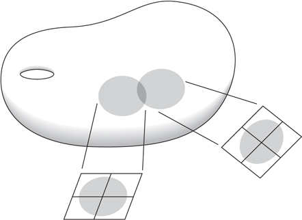
Figure 1 Small portions of a manifold resemble regions in a Euclidean space.

Figure 2 A transition function from a rectangulargrid to a distorted rectangular grid.

Now, here is a straightforward but central observation. Suppose that M and N are two neighborhoods that intersect, and suppose that functions ϕ : M → ^d and ψ: N → ^d are used to give them each a coordinate chart. Then the intersection M ∩ N is given two coordinate charts, and this gives us an identification between the open regions ϕ(M ∩ N) and ψ(M ∩ N) of ^d: given a point x in the first region, the corresponding point in the second is ψ(ϕ^-1(x)). This composition of maps is called a transition function, and it tells you how the coordinates from one of the charts on the intersecting region relate to those of the other. The transition function is a HOMEOMORPRISN [III.90] between the regions ϕ(M ∩ N) and ψ(M ∩ N).

Suppose that you take a rectangular grid in the first Euclidean region and use the transition function ψ ϕ^-1 to map it to the second one. It is possible that the image will again be a rectangular grid, but in general it will be somewhat distorted. An illustration is given in figure 2.

The proper term for a space whose points are surrounded by regions that can be identified with parts of Euclidean space is a topological manifold. The word “topological is used in order to indicate that there are no constraints on the coordinate-chart transition functions apart from the basic one that they should be continuous. However, some continuous functions are quite unpleasant, so one typically introduces extra constraints in order to limit the distorting effect that the transition functions can have on a rectangular coordinate grid.

Of prime interest here is the case where the transition functions are required to be differentiable to all orders. If a manifold has a collection of charts for which all the transition functions are infinitely differentiable, then it is said to have a smooth structure, and it is called a smooth manifold. Smooth manifolds are especially interesting because they are the natural arena for calculus. Roughly speaking, they are the most general context in which the notion of differentiation to any order makes intrinsic sense.

A function f, defined on a manifold, is said to be differentiable if, given any of its coordinate charts ϕ : N → ^d, the function g(y) = f(ϕ^-1(y)) (which is definedon a region of ^d) is DIFFERENTIABLE [I.3 § 5.3]. Calculusis impossible on a manifold if it does not admit chartswith differentiable transition functions, because a function that might appear differentiable in one chart willnot, in general, be differentiable when viewed from aneighboring chart.

Here is a one-dimensional example to illustrate this point. Consider the following two coordinate charts of a neighborhood of the origin in the real line. The first is the obvious chart that simply represents a real number x by itself. (Formally speaking, one is taking the function ϕ to be defined by the simple formula ϕ(x) = x.) The second represents x by the point x^1/3. (Here the cube root of a negative number x is defined to be minus the cube root of -x.) What is the transition function between these two charts? Well, if t is a point in the region of used for the first chart, then ϕ^-1 (t) = t, so ψ(ϕ^-1 (t)) = ψ(t) = t^1/3. This is a continuous function of t but it is not differentiable at the origin.

Now consider the simplest possible function defined on the region used for the second chart, the function h(s) = s, and let us work out the corresponding function f on the manifold itself. The value of f at x should be the value of h at the point s corresponding to x. This point is ψ(x) = x^1/3, so f(x) = h(x^1/3) = x^1/3. Finally, since the point x in the manifold corresponds to the point t = ϕ(x) = x in the first region, the corresponding function on the first region is g(t) = t^1/3 (This is the same function as f only because ϕ happens to be the very special map that takes each number to itself.) Thus, the eminently differentiable function h on one coordinate chart translates into the continuous but not differentiable function g on the other.

Suppose one is given a topological manifold M with two sets of charts, both of which have infinitely differentiable transition functions. Then each set of charts gives us a smooth structure on the manifold. Of great importance is the fact that these two smooth structures can be fundamentally different.

To see what this means, let us call the sets of charts K and L. Given a function f, let us call it K-differentiable if it is differentiable from the viewpoint of K, and L-differentiable if it is differentiable from the viewpoint of L. It may easily happen that a function is K-differentiable without being L-differentiable or vice versa. However, we can say that K and L give the same smooth structure on M when there is a map, F, from M to itself with the following three properties. First, F is invertible and both F and F^-1 are continuous. Second, the composition of F with any function that is K-differentiable is L-differentiable. Third, the composition of the inverse of F^-1 with any function that is L-differentiable is K-differentiable. Loosely speaking, F turns the K-differentiable functions into L-differentiable ones and F^-1 turns them back again. If no such function F exists, then the smooth structures given by K and L are considered to be genuinely different.

To see how this plays out, let us look at the one- dimensional example again. As noted previously, the functions that you deem to be differentiable if you use the ϕ-chart are not the same as those you deem to be differentiable if you use the ψ-chart. For example, the function x x^1/3 is not ϕ-differentiable but it is ψ-differentiable. Even so, the ϕ-differentiable and ψ-differentiable sets of functions define the same smooth structure for the line, since any ψ-differentiable function becomes ϕ-differentiable once you compose it with the self-map F : t t³.

It is very far from obvious that any manifold can have more than one smooth structure, but this turns out to be the case. There are also manifolds that are entirely lacking in smooth structures. These two facts lead directly to the central concern of this essay, the long-sought quest for the two holy grails of differential topology.

• A list of all smooth structures on any given topological manifold.
• An algorithm to identify any given smooth structure on any given topological manifold with the corresponding structure from the list.

2 What Is Known about Manifolds?

Much has been accomplished as of the writing of this article with respect to the two points listed above. This said, the task for this part of the article is to summarize the state of affairs at the beginning of the twenty-first century. Various examples of manifolds are described along the way.

The story here requires a brief, preliminary digression to set the stage. If you have two manifolds and you set them side by side without their touching, then technically speaking they can be regarded as a single manifold that happens to have two components. In such a case, one can study the components individually. Therefore, in this article I shall talk exclusively about connected manifolds: that is, manifolds with just one component. In a connected manifold, one can get from any point to any other point without ever leaving the manifold.

A second technical point is that it is useful to distinguish between manifolds such as the sphere, which are bounded in extent, and manifolds such as the plane, which go off to infinity More precisely, I am talking about the distinction between COMPACT [III.9] and non-compact manifolds: a compact manifold can be thought of as one that can be expressed as a closed bounded subset of ⁿ for some n. The discussion that follows will be almost entirely about compact manifolds. As some of the examples below will demonstrate, the story for compact manifolds is less convoluted than the analogous story for noncompact ones. For simplicity I shall often use the word “manifold”; to mean “compact manifold; it will be clear from the context if noncompact manifolds are also being discussed.

2.1 Dimension 0

There is only one dimension-0 manifold. It is a single point. The period at the end of this sentence looks, from afar, like a connected, dimension-0 manifold. Note that the distinction between topological and smooth is irrelevant here.

Figure 3 Two charts that cover the circle.

2.2 Dimension 1

There is only one compact, connected, one-dimensional topological manifold, namely the circle. Moreover, the circle has just one smooth structure. Here is one way to represent this structure. Take as a representative circle the unit circle in the xy-plane, that is, the set of all points (x,y) with x² + y² = 1. This can be covered by two overlapping intervals, each of which covers slightly more than half of the circle. The intervals U₁ and U₂ are drawn in figure 3. Each interval constitutes a coordinate chart. The one on the left, U₁, can be parametrized in a continuous fashion by taking the angle of a given point as measured counterclockwise from the positive x-axis. For example, the point (1,0) has angle 0, and the point (-1, 0) has angle π. In order to parametrize U₂ by angle, you will have to start with angle π at the negative x-axis. If you move around U₂, varying this angle continuously, then when you reach the point (1, 0) you will have parametrized it as a point in U₂ using the angle 2π.

As you can see, the arcs U₁ and U₂ intersect in two separated, smaller arcs; these are labeled V₁ and V₂ in figure 4. The transition function on V₁ is the identity map, since the U₁ angle of any given point in V₁ is the same as its U₂ angle. By contrast, the U₂ angle of a point in V₂ is obtained from the U₁ angle by adding 2π. Thus, the transition function on V₂ is not the identity map but the map that adds 2π to the coordinate function.

This one-dimensional example brings up a number of important issues, all related to a particularly troubling question. To state it, consider first that there are lots of closed loops in the plane that can be taken as model circles. Indeed, the word “lots” considerably understates the situation. Moreover, why should we restrict our attention to circles in the plane? There are closed loops galore in 3-space too: see figure 5, for example. For that matter, any manifold of dimension greater than 1 has smooth loops. Earlier, it was asserted that there is just one smooth, compact, connected, one-dimensional manifold, so all of these loops must be considered the “same.” Why is this?

Figure 4 The intersection of the arcs U₁ and U₂.

Figure 5 A knotted loop in 3-space.

Here is the answer. We often think of a manifold as it might appear were it sitting in some larger space. For example, we might imagine a circle sitting in the plane, or sitting knotted in three-dimensional Euclidean space. However, the notion of “smooth manifold” introduced above is an intrinsic one, in the sense that it does not depend on how the manifold is placed inside a higher-dimensional space. Indeed, it is not even necessary for there to be a higher-dimensional space at all. In the case of the circle, this can be said in the following way. The circle can be placed as a loop in the plane, or as a knot in 3-space, or whatever. Each view of the circle in a higher-dimensional Euclidean space defines a collection of functions that are considered differentiable: one just takes the differentiable functions of the coordinates of the big Euclidean space and restricts them to the circle. As it turns out, any one such collection defines the same smooth structure on the circle as any other. Thus, the smooth structures that are provided by these different views of a circle are all the same, even though there are many interesting ways of placing a circle in a given higher-dimensional space. (In fact, the classification of knots in 3-space is a fascinating, vibrant topic in its Own right: see KNOT POLYNOMIALS [III.44].)

Figure 6 A Möbius strip has just one side.

How is it proved that there is only one smooth structure for the circle? For that matter, how is it proved that there is but a single compact topological manifold in dimension 1? Since this article is not meant to provide proofs, these questions are left as serious exercises with the following advice. Think hard about the definitions and, for the smooth-manifold question, use some calculus.

2.3 Dimension 2

The story for two-dimensional, connected, compact manifolds is much richer than that for dimension 1. In the first place, there is a basic dichotomy between two kinds of manifold: orientable and nonorientable. Roughly speaking, this is the distinction between manifolds that have two sides and those that have just one. To give a more formal definition, a two-dimensional manifold is called orientable if every loop in the manifold that does not cross itself or have any kinks has two distinct sides. This is to say that there is no path from one side of the loop to the other that avoids the loop yet remains very close to it. The Möbius strip (see figure 6) is not orientable because there are paths from one side of the central loop to the other that do not cross the central loop yet remain very close to it. The orientable, compact, connected, topological, two-dimensional manifolds are in one-to-one correspondence with a collection of fundamental foods: the apple, the doughnut, the two-holed pretzel, the three- holed pretzel, the four-holed pretzel, and so on (see figure 7). Technically, they are classified by an integer, called the genus. This is 0 for the sphere, 1 for the torus, 2 for the two-holed torus, etc. The genus counts the number of holes that appear in a given example from figure 7. To say that this classifies them is to say that two such manifolds are the same if and only if they have the same genus. This is a theorem due to POINCARÉ [VI.61].

Figure 7 The orientable manifolds of dimension 2.

Figure 8 Cutting and gluing.

As it turns out, every topological two-dimensional manifold has exactly one smooth structure, so the list in figure 7 is the same as the list of the smooth orientable two-dimensional manifolds. Here one should keep in mind that the notion of a smooth manifold is intrinsic, and therefore independent of how the manifold is represented as a surface in 3-space, or in any other space. For example, the surfaces of an orange, a banana, and a watermelon each represent embedded images of the two-dimensional sphere, the leftmost example in figure 7.

The shapes illustrated in figure 7 suggest an idea that plays a key role when it comes to classifying manifolds of higher dimensions. Notice that the two-holed torus can be viewed as the result of taking two one-holed tori, cutting disks out of both, gluing the results together across their boundary circles, and then smoothing the corners. This operation is depicted in figure 8. This sort of cutting and gluing operation is an example of what is called a surgery. The analogous surgery can also be done with a one-holed torus and a two-holed torus to obtain a three-holed torus. And so on. Thus, all of the oriented two-dimensional manifolds can be built using standard surgeries on copies of just two fundamental building blocks: the one-holed torus and the sphere. Here is a nice exercise to test your understanding of this process. Suppose that you perform a surgery, as in figure 8, on a sphere and another manifold M. Prove that the resulting manifold is the same, with regard to its topological and smooth structure, as M.

As it turns out, all of the nonorientable two-dimensional manifolds can be built using a version of surgery that first cuts a disk out of an orientable two-dimensional manifold and then glues on a Möbius strip. To be more precise, note that the Möbius strip has a circle as its boundary. Cut a disk out of any given orientable, two-dimensional manifold and the result also has a circular boundary. Glue the latter circular boundary to the Möbius strip boundary, smooth the corners, and the result is a smooth manifold that is nonorientable. Every nonorientable, topological (and thus every nonorientable, smooth), two-dimensional manifold is obtained in this way. Moreover, the manifold you get depends only on the number of holes (the genus) of the orientable manifold that is used.

Figure 9 Two nonorientable surfaces. To form the projective plane, one identifies the boundary of the Möbius strip with the boundary of the hemisphere.

The manifold obtained from the surgery of a Möbius strip with a sphere is called the projective plane. The one that uses the Möbius strip and the torus is called the Klein bottle. These shapes are illustrated in figure 9. No nonorientable example can be put into three-dimensional Euclidean space in a clean way; any such placement is forced to have portions that pass through other portions, as can be seen in the illustration of the Klein bottle.

How does one prove that the list given above exhausts all two-dimensional manifolds? One method uses versions of the geometric techniques that are discussed below in the three-dimensional context.

2.4 Dimension 3

There is now a complete classification of all smooth, three-dimensional manifolds; however, this is a very recent achievement. There has been for some time a conjectured list of all three-dimensional manifolds, and a conjectured procedure for telling one from the other. The proof of these conjectures was recently completed by Grigori Perelman; this is a much-celebrated event in the mathematics community. The proof uses geometry about which more is said in the final part of this article. Here I shall concentrate on the classification scheme.

Before getting to the classification scheme, it is necessary to introduce the notion of a geometric structure on a manifold. Roughly speaking, this means a rule for defining the lengths of paths on the manifold. This rule must satisfy the following conditions. The constant path that simply stays at one point has length 0, but any path that moves at all has positive length. Second, if one path starts where another ends, the length of their concatenation (that is, the result of putting the two paths together) is the sum of their lengths.

Note that a rule of this sort for path lengths leads naturally to a notion of distance d(x,y) between any two points x and y on the manifold: one takes the length of the shortest path between them. It turns out to be particularly interesting when d(x,y)² varies as a smooth function of x and y.

As it happens, there is nothing special about having a geometric structure. Manifolds have them in spades. The following are three very useful geometric structures for the interior of the ball of radius 2 about the origin in n-dimensional Euclidean space. In these formulas, the given path is viewed as if drawn in real time by some hyper-dimensional artist, with x(t) denoting the position of the pencil tip on the path at time t. Here, t ranges over some interval of the real line:

In these formulas, denotes the time-derivative of the path t x(t).

The first of these geometric structures leads to the standard Euclidean distance between pairs of points. For this reason it is called the Euclidean geometry for the ball. The second defines what is called spherical geometry because the distance between any two points is the angle between certain corresponding points in the sphere of radius 1 in (n + 1)-dimensional Euclidean space. The correspondence comes from an (n + 1)-dimensional version of the stereographic projection that is used for maps of the Earth’s polar regions. The third distance function defines what is called the hyperbolic geometry on the ball. This arises when the ball of radius 2 in n-dimensional Euclidean space is identified in a certain way with a particular hyperbola in (n + 1)-dimensional Euclidean space.

The geometric structures that are depicted in (1) turn out to be symmetrical with respect to rotations and certain other transformations of the unit ball. (You can read more about Euclidean, spherical, and hyperbolic geometry in SOME FUNDAMENTAL MATHEMATICAL DEFINITIONS [I.3 §§6.2, 6.5, 6.6].)

As was remarked above, there are very many geometric structures on any given manifold and so one might hope to find one that has some particularly desirable properties. With this goal in mind, suppose that I have specified some “standard” geometric structure S for the ball in ⁿ to serve as a model of an exceptionally desirable structure. This could be one of the ones I have just defined or some other favorite. This leads to a corresponding notion of the structure S for a compact manifold. Roughly speaking, one says that a geometric structure on a manifold is of the type S if every point in the manifold feels as though it belongs to the unit ball with the structure S, that is, if one can use the structure S on the ball to provide coordinate charts that respect the geometric structure on the manifold. To be more precise, suppose that I am defining a coordinate system in a small neighborhood N of x by means of a function ϕ : N → ^d. If I can always do this in such a way that the image ϕ(N) lies inside the ball, and such that the distance between any two points x and y in N equals the distance between their images ϕ(x) and ϕ(y), defined in terms of the structure S on the ball, then I will say that the manifold has structure of type S. In particular, a geometric structure is said to be Euclidean, spherical, or hyperbolic when the structure on the ball is Euclidean, spherical, or hyperbolic, respectively.

For example, the sphere in any dimension has a spherical geometric structure (as it should!). As it turns out, every two-dimensional manifold has a geometric structure that is either spherical, Euclidean, or hyperbolic. Moreover, if it has a structure of one of these types, then it cannot have one of a different type. In particular, the sphere has a spherical structure, but not a Euclidean or hyperbolic structure. Meanwhile, the torus in dimension 2 has a Euclidean geometric structure but only a Euclidean one, and all of the other manifolds listed in figure 7 have hyperbolic geometric structures and only hyperbolic ones.

William Thurston had the great insight to realize that three-dimensional manifolds might be classifiable using geometric structures. In particular, he made what was known as the geometrization conjecture, which says, roughly speaking, that every three-dimensional manifold is made up of “nice” pieces:

Every smooth three-dimensional manifold can be cut in a canonical fashion along a predetermined set of two- dimensional spheres and one-holed tori so that each of the resulting parts has precisely one of a list of eight possible geometric structures.

The eight possible structures include the spherical, Euclidean, and hyperbolic ones. These plus the other five are, in a sense that can be made precise, those that are maximally symmetric. The other five are associated with various LIE GROUPS [III.48 § 1], as are the listed three.

Since its proof by Perelman, the geometrization conjecture has come to be known as the geometrization theorem. As I shall explain in a moment, this provides a satisfactory resolution of the three-dimensional part of the quest set out at the end of section 1. This is because a manifold with one of the eight geometric structures can be described in a canonical fashion using group theory. As a result, the geometrization theorem turns the classification issue for manifolds into a question that group theory can answer. What follows is an indication of how this comes about.

Each of the eight geometric structures has an associated model space which has the given geometric structure. For example, in the case of the spherical structure, the model space is the three-dimensional sphere. For the Euclidean structure, the model space is the three- dimensional Euclidean space. For the hyperbolic structure, it is the hyperbola in the four-dimensional Euclidean space, where the coordinates (x,y,z,t) obey t² = 1 + x² + y² + z². In all of the eight cases, the model space has a canonical group of self-maps that preserve the distance between any two pairs of points. In the Euclidean case, this group is the group of translations and rotations of the three-dimensional Euclidean space. In the spherical case, it is the group of rotations of the four-dimensional Euclidean space, and in the hyperbolic case, it is the group of Lorentz transformations of four-dimensional Minkowski space. The associated group of self-maps is called the isometry group for the given geometric structure.

The connection between manifolds and group theory arises because a certain set of discrete subgroups of the isometry group of any one of the eight model spaces determines a compact manifold with the corresponding geometric structure. (A subgroup is called discrete if every point in the subgroup is isolated, meaning that it belongs to a neighborhood that contains no other points from the subgroup.) This compact manifold is obtained as follows. Two points x and y in the model space are declared to be equivalent if there is an isometry T, belonging to the subgroup, such that Tx = y. In other words, x is equivalent to all its images under isometrics from the subgroup. It is easy to check that this notion of equivalence is a genuine EQUIVALENCE RELATION [I.2 §2.3]. The equivalence classes are then in one-to-one correspondence with the points of the associated compact manifold.

Here is a one-dimensional example of how this works. Think of the real line as a model space whose isometry group is the group of translations. The set of translations by integer multiples of 2π forms a discrete subgroup of this group. Given a point t in the real line, the possible images under translations from the subgroup are all the numbers of the form t + 2nπ, where n is an integer, so one regards two real numbers as equivalent if they differ by a multiple of 2π, and the equivalence class of t is {t + 2nπ : n ∈ }. One can associate with this equivalence class the point (x,y) = (cos t, sin t) in the circle, since adding a multiple of 2π to t does not affect either its sine or its cosine. (Intuitively speaking, if you regard each t as equivalent to t + 2π, then you are wrapping the real line around and around a circle.)

This association between certain subgroups of the isometry group and compact manifolds with the given geometric structure goes in the other direction as well. That is, the subgroup can be recovered from the manifold in a relatively straightforward fashion using the fact that each point in the manifold lies in a coordinate chart where its distance function is the same as that of the associated model space.

Even before Perelman’s work there was a tremendous amount of evidence for the validity of the geometrization conjecture, much of it supplied by Thurston. In order to discuss this evidence, a small digression is required to give some of the background. First, I need to bring in the notion of a link in the three-dimensional sphere. A link is the name given to a finite disjoint union of knots. figure 10 depicts an example of one that is made out of two knots.

Figure 10 A link formed out of two knots.

I also need the notion of surgery on a link. To this end, thicken the link so as to view it as a union of knotted, solid tubes. (Think of the knot as the copper in an insulated wire and view the solid tube as the copper plus the surrounding insulation.) Notice that the boundary of any given component tube is really a copy of our one-holed torus from figure 7. Therefore, removing any one of the tubes leaves a tubular-shaped missing region from the three-dimensional sphere whose boundary is a torus.

Now, to define a surgery, imagine removing a knotted tube and then gluing it back in a different way. That is, imagine gluing the boundary of the tube to the boundary of the resulting missing region using an identification that is not the same as the original. For example, take the “unknot,” a standard round circle in a given plane, here viewed as living inside a coordinate chart of the three-dimensional sphere. Take out the solid tube around it, and then replace the tube by gluing the boundary in the “wrong” way, as follows. Consider the leftmost torus in figure 11 as the boundary of the complement of the tube in ³. Consider the middle torus as the inside of the tube. The “wrong” gluing identifies the circles marked “R” and “L” on the leftmost torus with their counterparts on the middle torus. The resulting space is a three-dimensional manifold which turns out to be the product of the circle with the two-dimensional sphere. That is to say, it is the set of ordered pairs (x,y), where x is a point in the circle and y is a point in the two-dimensional sphere. There are many other possible ways to glue the boundary torus, and almost all of the corresponding surgeries give rise to distinct three-dimensional manifolds. One of these is illustrated in the rightmost part of figure 11.

In general, given any link one can construct a count- ably infinite set of distinct, smooth three-dimensional manifolds by using surgeries on it. Furthermore, Raymond Lickorish proved that every three-dimensional manifold can be obtained by using surgery on some link in the three-dimensional sphere. Unfortunately, this characterization of three-dimensional manifolds via surgeries on links does not provide a satisfactory resolution to the central quest of classifying smooth structures because the process is far from unique: for any given manifold there is a bewildering assortment of links and surgeries that can be used to produce it. Moreover, as of this writing, there is no known way to classify knots and links in the three-dimensional sphere.

In any event, here is a taste of Thurston’s evidence for his geometrization conjecture. Given any link, all but finitely many of the three-dimensional manifolds you can produce from it by surgery satisfy the conclusions of the geometrization conjecture. Thurston also proved that, given any knot apart from the unknot, all but finitely many surgeries on it produce a manifold with a hyperbolic geometric structure.

By the way, Perelmans proof of the geometrization theorem gives as a special case a proof of the Poincaré conjecture, proposed by Poincgré in 1904. To state this we need the notion of a simply connected manifold. This is a manifold with the property that any closed loop in it can be shrunk down to a point. To be more precise, designate a point in the manifold as the “base point.” Then any path in the manifold that starts and ends at the chosen base point can be continuously deformed in such a way that at each stage of the deformation the path still starts and ends at the base point, and so that the end result is the trivial path that starts at the base point and just stays there. For example, the two- dimensional sphere is simply connected, but the torus is not, since a loop that goes “once around” the torus (for example, any of the loops R or L in the various tori of figure 11) cannot be shrunk to a point. In fact, a sphere is the only two-dimensional manifold that is simply connected, and spheres are simply connected in all dimensions greater than 1.

The Poincaré conjecture. Every compact, simply connected, three-dimensional manifold is the three-dimensional sphere.

2.5 Dimension 4

This is the weird dimension. Nobody has managed to formulate a useful and viable conjecture for the classification of smooth, compact, four-dimensional manifolds. On the other hand, the classification story for many categories of topological four-dimensional manifolds is well-understood. For the most part, this work is by Michael Freedman.

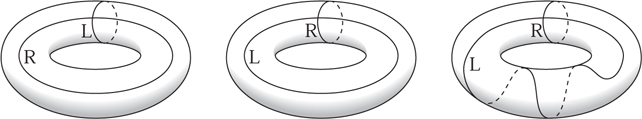
Figure 11 Different ways of gluing a tube into a tube-shaped hole.

Some of the topological manifolds in dimension 4 do not admit smooth structures. The so-called “ conjecture” proposes necessary and sufficient conditions for a four-dimensional, topological manifold to have at least one smooth structure. The fraction here refers to the absolute value of the ratio of the rank to the signature of a certain symmetric, bilinear form that appears in the four-dimensional story. The case excepted, the conjecture asserts that a smooth structure exists if and only if this ratio is at least . The bilinear form in question is obtained by counting with signed weights the intersection points between various two-dimensional surfaces inside the given four- dimensional manifold. In this regard, note that a typical pair of two-dimensional surfaces in four dimensions will intersect at finitely many points. This is a higher- dimensional analogue of a fact that is rather easier to visualize: that a typical pair of loops in the two-dimensional plane will intersect at finitely many points. Not surprisingly, the bilinear form here is called the intersection form; it plays a prominent role in Freedman’s classification theorems.

Meanwhile, the problem of listing all smooth structures is wide open in four dimensions: there are no cases of a topological manifold with at least one smooth structure where the list of distinct structures is known to be complete. Some topological four- dimensional manifolds are known to have (countably) infinitely many distinct smooth structures. For others there is only one known structure. For example, the four-dimensional sphere has one obvious smooth structure and this is the only one known. However, the underlying topological manifold may, for all anyone knows, have many distinct smooth structures. By the way, the story for noncompact manifolds in dimension 4 is truly bizarre. For example, it is known that there are uncountably many smooth manifolds that are homeomorphic to the standard, four-dimensional Euclidean space. But even here, our understanding is less than optimal since there is no known explicit construction of a single one of these “exotic” smooth structures.

Simon Donaldson provided a set of geometric invariants that have the power to distinguish smooth structures on a given topological 4-manifold. Donaldson’s invariants were recently superseded by a suite of more computable invariants; these were proposed by Edward Witten and are called the Seiberg-Witten invariants. More recently still, Peter Oszvath and Zoltan Szabo designed a possibly equivalent set of invariants that are even easier to use. Do the Seiberg–Witten invariants (broadly defined) distinguish all smooth structures? No one knows. ? bit more is said about these invariants in the final part of this article.

Note that Freedman’s results include the topological version of the four-dimensional Poincaré conjecture that follows.

The four-dimensional sphere is the only compact, topological 4-manifold with the following property: every based map from either a one-dimensional circle or a two-dimensional sphere can be continuously deformed so that the result maps onto the base point.

The smooth version of this conjecture has not been resolved.

Is there a four-dimensional version of the geometrization conjecture/theorem?

2.6 Dimensions 5 and Greater

Surprisingly enough, the issues raised at the end of the first section have more or less been resolved in all dimensions that are greater than 4. This was done some time ago by Stephen Smale with input from John Stallings. In these higher dimensions it is also possible to say what conditions need to hold in order for a topological manifold to admit a smooth structure. For example, John Milnor and others determined that the respective number of smooth structures on the spheres of dimensions 5–18 are as follows: 1, 1, 28, 2, 8, 6, 992, 1, 3, 2, 16, 256, 2, 16, 16.

At first sight, it is surprising that the dimensions greater than 4 are easier to deal with than dimensions 3 and 4. However, there is a good reason for this. It turns out that there is more room to maneuver in these higher-dimensional spaces and this extra room makes all the difference. To get a sense for this, let n be a positive integer, and let Sⁿ denote the n-dimensional sphere. To make this more concrete, view Sⁿ as the set of points (x₁, . . . ,x_{n + 1}) in the Euclidean space ⁿ such that + . . . + = 1. Now consider the product manifold, Sⁿ × Sⁿ. This is the set of pairs of points (x,y), where x is in one copy of Sⁿ and y is in another. This product manifold has dimension 2n. A standard picture of Sⁿ × Sⁿ has two distinguished copies of Sⁿ inside it, one consisting of all points of the form (x,y) with y = (1, 0,. . .) and the other consisting of all points (x,y) with x = (1,0,. . .). Let us call the first copy S_R and the second one S_L. Of particular interest here is the fact that S_R and S_L intersect in precisely one point, the point ((1, 0, . . .), (1, 0, . . .)).

By the way, in the n = 1 case, the space S¹ × S¹ is the doughnut in figure 7. The one-dimensional spheres S_R and S_L inside it are the circles that are drawn in the leftmost diagram in figure 11.

If you are with me so far, suppose now that an advanced alien en route from Arcturus to the galactic center kidnaps you and drops you into some unknown, 2n-dimensional manifold. You suspect that it is Sⁿ × Sⁿ, but are not sure. One reason that you suspect this to be the case is that you have found a pair of n-dimensional spheres in it, one you call M_R and the other you call M_L. Unfortunately, they intersect in 2N + 1 points, where N > 0. You would be less nervous about things if you could find a pair of different spheres that intersect precisely once. So you wonder whether perhaps you can push M_L around a bit so as to remove the 2N unwanted intersection points.

The surprise here is that the issue of removing intersection points in any dimension concerns only certain zero-, one-, and two-dimensional manifolds that live inside your 2n-dimensional one. This is an old observation due to Hassler Whitney. In particular, Whitney discovered that in the 2n-dimensional manifold you must be able to find a disk of dimension two whose boundary loop lies half in M_L and half in M_R. This boundary loop must hit two of the intersection points (one when it passes from M_L to M_R and one when it passes back again). The disk must also stick out orthogonally to M_L and M_R where it touches them. If its interior is disjoint from both M_L and M_R, and if there are no points where the disk comes back to intersect itself, then you can push the part of M_L that is very near the disk along the disk while stretching the remaining part to keep things from tearing. If you extend the disk a bit past M_R, then you will have removed two of the intersection points when you have pushed past the end of the disk. figure 12 is a schematic of this. This pushing operation (the Whitney trick) can be performed in any manifold of any dimension if you can find the required disk. The problem is to find the disk. figure 13 is a drawing of a cross-sectional slice showing a “good” disk on the left and some badly chosen disks in the middle and on the right. If you have a badly chosen disk that nevertheless satisfies the required boundary conditions, then you might hope to find a tiny wiggle of its interior that makes it better. You would like the new disk to have no self-intersection points and you would like its interior to be disjoint from both M_L and M_R. No wiggle along a direction that is parallel to the disk itself will help, for any such wiggle only changes the position of the intersection point in the disk. Likewise, a wiggle in a direction parallel to the offending M_L or M_R is useless since it only changes the position of the intersection point in the latter space. Thus, 2 + n of the 2n dimensions are useless when it comes to wiggling a disk. However, there are 2n - (n + 2) = n - 2 remaining dimensions to work with, which is a positive number when 2n > 4. In fact, when this is true a generic wiggle in any of these extra dimensions does the trick.

Now, when 2n = 4 (so n = 2) there are no extra dimensions, and, consequently, no small wiggle can make a new disk without intersection points. So if a given candidate disk intersects M_R, then the Whitney trick just trades the old pair of intersection points for a new collection. If the disk intersects either itself or M_L, then the new version of M_L has self-intersection points: that is, points where one part has come around to intersect another.

This failure of the Whitney trick is the bane of four-dimensional topology. Thus, a major lemma for Michael Freedman’s classification theorem about topological four-dimensional manifolds describes ubiquitous circumstances where a topologically (but not smoothly!) embedded disk can be found for use in the Whitney trick.

3 How Geometry Enters the Fray

Much of our current understanding about smooth manifolds in dimensions 4 or less has come via what might be called geometric techniques. The search for a canonical geometric structure on a given three-dimensional manifold is an example. Perelman’s proof of the geometrization theorem proceeds in this manner. The idea is to choose any convenient geometric structure on a given three-dimensional manifold and then continuously deform it by some well-defined rule. If one views the deformation as a time-dependent process, then the goal is to design the deformation rule to make the geometric structure ever more symmetric as time goes on.

Figure 12 The Whitney trick.

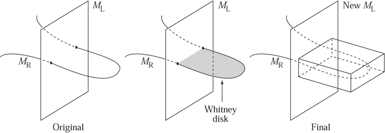
Figure 13 Some possible Whitney disks.

A rule introduced and much studied by Richard Hamilton and then used by Perelman specifies the time-derivative of the geometric structure at any given time in terms of certain of its properties at that time. It is a nonlinear version of the classical HEAT EQUATION [I.3 §5.4]. For those unfamiliar with the latter, the simplest version modifies functions on the real line and will now be described. Let τ denote the time parameter, and let f(x) denote a given function on the line, representing the initial distribution of heat. The resulting time-dependent family of functions associates with any given positive value for τ a function, F_τ(x), which represents the distribution of heat at time τ. The partial derivative of F_τ(x) with respect to τ is equal to its second partial derivative with respect to x, and the initial condition is that F₀(x) = f(x). If the initial function f is zero outside some interval, then one can write down a formula for F_τ:

One can see from (2) that F_τ(x) tends uniformly to zero in x as τ tends to infinity In particular, this limit is completely ignorant of the starting function f; and, being identically zero, it is also the most symmetric function possible. The representation for F_τ in (2) indicates how this comes about. The value of F_τ at any given point is a weighted average of the values of the original function. Moreover, as τ increases, this average looks more like the standard average over ever-larger regions of the line. Physically this is very plausible as well: the heat spreads itself out more and more thinly as time goes on.

The time-dependent family of geometric structures that Hamilton introduced and Perelman used is defined by an equation that relates the time-derivative of the geometric structure at any given time to its Ricci curvature, a certain natural substitute in the context of geometric structures for the second derivatives that enter the heat equation for the functions F_τ above. The idea much studied by Hamilton and then by Perelman is to let the evolving geometric structure decompose the manifold into the canonical pieces that are predicted to exist by the geometrization conjecture. Perelman proved that the pieces required by the geometrization conjecture emerge as regions whose points stay relatively close together (as measured by a certain rescaling of the distance function) while the points in distinct regions move farther and farther apart.

The equation used by Perelman and Hamilton for the time-evolution of a geometric structure is rather complicated. Its standard incarnation involves the notion of a RIEMANNIAN METRIC [I.3 §6.10]. This appears in any given coordinate chart on an n-dimensional manifold as a symmetric, positive-definite n × n matrix whose entries are functions of the coordinates. The various components of this matrix are traditionally written as {g_ij}_{1≤i, j≤n}. The matrix determines the geometric structure and can in turn be derived from it.

Hamilton and Perelman study a time-dependent family of Riemannian metrics, τ → g_τ, where the rule for the time dependence is obtained using an equation for the τ-derivative of g_τ that has the schematic form ∂_τ(g_τ)_i,j = - 2R_i,j[g_τ], where {R_{i j}}_{1 ≤i, j≤n} are the components of the aforementioned Ricci curvature, a certain symmetric matrix that is determined at any given τ by the metric g_τ. Every Riemannian metric has a Ricci curvature; its components are standard (nonlinear) functions of the components of the matrix and their first- and second-order partial derivatives in the coordinate directions. The Ricci curvatures for the metrics that define the respective Euclidean, spherical, and hyperbolic geometries have the particularly simple form R_{i j} = cg_{i j}, where c is 0, 1, or -1, respectively. For more about these ideas, see RICCI FLOW [III.78].

As was mentioned at the beginning of this part of the article, geometry has also played a central role in the developments in the classification program for smooth, four-dimensional manifolds. In this case, geometrically defined data are used to distinguish smooth structures on topologically equivalent manifolds. What follows is a very brief sketch of how this is done.

To begin with, the idea is to introduce a geometric structure on the manifold and then to use the latter to define a canonical system of partial differential equations. In any given coordinate chart, these equations are for a particular set of functions. The equations state that certain linear combinations of the collection of first derivatives of the functions from the set are equal to terms that are linear and quadratic in the values of the functions themselves. In the case of the Donaldson invariants, and also of the newer Seiberg–Witten invariants, the relevant equations are nonlinear generalizations of the MAXWELL EQUATIONS [IV.13 §1.1] for electricity and magnetism.

In any event, one then counts the solutions with algebraic weights. The purpose of the algebraic weighting of the count is to obtain an INVARIANT [I.4 §2.2], that is, a count that does not change if the given geometric structure is changed. The point here is that the naive count will typically depend on the structure, but a suitably weighted count will not. Imagine, for example, that one has a continuously varying family of geometric structures, and that new solutions appear and old ones disappear only in pairs, where one solution has been assigned weight +1 and the other -1.

The following toy model illustrates this appearance and disappearance phenomenon. The equation in question is for a single function on the circle. That is, it will concern a function, f, of one variable, x, that is periodic with period 2π. For example, take the equation ∂f/∂x + τf - f³ = 0, where τ is a constant that is specified in advance. Varying τ can now be viewed as a model for the variation of the geometric structure. When τ > 0 there are exactly three solutions: f ≡ 0, f ≡ τ, and f ≡ -τ. However, when τ ≤ 0, the only solution is f ≡ 0. Thus, the number of solutions changes as τ crosses zero. Even so, a suitable weighted count is independent of τ.

Let us return now to the four-dimensional story. If the weighted sum is independent of the chosen geometric structure, then it depends only on the underlying smooth structure. Therefore, if two geometric structures on a given topological manifold provide distinct sums, then the underlying smooth structures must be distinct.

As I remarked earlier, Oszvath and Szabo have defined invariants for four-dimensional manifolds that are easier to use than the Seiberg-Witten invariants, but probably equivalent to them. These are also defined as the number of solutions to a particular system of differential equations, counted in a creative way. In this case, the equations are analogues of the CAUCHY–RIEMANN EQUATIONS [I.3 §5.6], and the arena is a space that can be defined after cutting the 4-manifold into simpler pieces. There are myriad ways to slice a 4-manifold in the prescribed manner, but a suitably creative, algebraic count of solutions provides the same number for each.

With hindsight, one can see that the use of differential equations to distinguish smooth structures on a given topological manifold makes good sense, since a smooth structure is needed to take a derivative in the first place. Even so, this author is constantly amazed by the fact that the Donaldson/Seiberg-Witten/Oszvath-Szabo strategy of algebraically counting differential equation solutions yields counts that are both tractable and useful. (Getting the same count in all cases is no help at all.)

Further Reading

Those who wish to learn more about manifolds in general can consult J. Milnor’s book Topology from the Differentiable Viewpoint (Princeton University Press, Princeton, NJ, 1997) or the book Differential Topology (Prentice Hall, Englewood Cliffs, NJ, 1974), by V. Guillemin and A. Pollack. A good introduction to the classification problem in dimensions 2 and 3 is the book Three-Dimensional Geometry and Topology (Princeton University Press, Princeton, NJ, 1997), by W. Thurston. This book also has a nice discussion of geometric structures. A full account of Perelman’s proof of the Poincaré conjecture can be found in Ricci Flow and the Poincaré Conjecture, by J. Morgan and G. Tian (American Mathematical Society, Providence, RI, 2007). The story for topological 4-manifolds is told in the book by M. Freedman and F. Quinn titled Topology of 4-Manifolds (Princeton University Press, Princeton, NJ, 1990). There are no books available that serve as general introductions to the smooth 4-manifold story. A book that does introduce the Seiberg-Witten invariants is The Seiberg-Witten Equations and Applications to the Topology of Smooth Four-Manifolds (Princeton University Press, Princeton, NJ, 1995), by J. Morgan. Meanwhile, the Donaldson invariants are discussed in detail in the book by Donaldson and P. Kronheimer titled Geometry of Four-Manifolds (Oxford University Press, Oxford, 1990). Finally, parts of the story for dimensions greater than 4 are told in Lectures on the h-Cobordism Theorem (Princeton University Press, Princeton, NJ, 1965), by J. Milnor, and Foundational Essays on Topological Manifolds, Smoothings and Triangulcitions (Princeton University Press, Princeton, NJ, 1977), by R. Kirby and L. Siebenman.