
IV.22 Set Theory
Joan Bagaria
1 Introduction
Among all mathematical disciplines, set theory occupies a special place because it plays two very different roles at the same time: on the one hand, it is an area of mathematics devoted to the study of abstract sets and their properties; on the other, it provides mathematics with its foundation. This second aspect of set theory gives it philosophical as well as mathematical significance. We shall discuss both aspects of the subject in this article.
2 The Theory of Transfinite Numbers
Set theory began with the work of CANTOR [VI.54]. In 1874 he proved that there are more real numbers than there are algebraic ones, thus showing that infinite sets can be of different sizes. This also provided a new proof of the existence of TRANSCENDENTAL NUMBERS [III.41]. Recall that a real number is called algebraic if it is the solution of some polynomial equation
anXn + an-1Xn-1 + · · · + a1X + a0 = 0,
where the coefficients ai are integers (and an ≠ 0). Thus, numbers like ![]() ,
, ![]() , and the golden ratio,
, and the golden ratio, ![]() (1 +
(1 + ![]() ), are algebraic. A transcendental number is one that is not algebraic.
), are algebraic. A transcendental number is one that is not algebraic.
What does it mean to say that there are “more” real numbers than algebraic ones, when there are infinitely many of both? Cantor defined two sets A and B to have the same size, or cardinality, if there is a bijection between them: that is, if there is a one-to-one correspondence between the elements of A and the elements of B. If there is no bijection between A and B, but there is a bijection between A and a subset of B, then A is of smaller cardinality than B. So what Cantor in fact showed was that the set of algebraic numbers had smaller cardinality than that of all real numbers.
In particular, Cantor distinguished between two different kinds of infinite set: COUNTABLE AND UNCOUNTABLE [III.11]. A countable set is one that can be put into one-to-one correspondence with the natural numbers. In other words, it is a set that we can “enumerate,” assigning a different natural number to each of its elements. Let us see how this can be done for the algebraic numbers. Given a polynomial equation as above, let the number
|an| + |an-1| + · · · + |a0| + n
be called its index. It is easy to see that for every k > 0 there are only a finite number of equations of index k. For instance, there are only four equations of index 3 with strictly positive an, namely, X2 = 0, 2X = 0, X + 1 = 0, and X - 1 = 0, which have as solutions 0, -1, and 1. Thus, we can enumerate the algebraic numbers by first enumerating all solutions of equations of index 1, then all solutions of equations of index 2 that we have not already enumerated, and so on. Therefore, the algebraic numbers are countable. Note that from this proof we also see that the sets ![]() and
and ![]() are countable.
are countable.
Cantor discovered that, surprisingly, the set ![]() of real numbers is not countable. Here is Cantor’s original proof. Suppose, aiming for a contradiction, that r0, r1, r2, . . . is an enumeration of
of real numbers is not countable. Here is Cantor’s original proof. Suppose, aiming for a contradiction, that r0, r1, r2, . . . is an enumeration of ![]() . Let a0 = r0. Choose the least k such that a0 < rk and put b0 = rk. Given an and bn, choose the least l such that an < rl < bn, and put an + 1 = rl. And choose the least m such that an+1 < rm < bn, and put bn+1 = rm. Thus, we have a0 < a1 < a2 < · · · < b2 < b1 < b0. Now let a be the limit of the an. Then a is a real number different from rn, for all n, contradicting our assumption that the sequence r0, r1, r2, . . . enumerates all real numbers.
. Let a0 = r0. Choose the least k such that a0 < rk and put b0 = rk. Given an and bn, choose the least l such that an < rl < bn, and put an + 1 = rl. And choose the least m such that an+1 < rm < bn, and put bn+1 = rm. Thus, we have a0 < a1 < a2 < · · · < b2 < b1 < b0. Now let a be the limit of the an. Then a is a real number different from rn, for all n, contradicting our assumption that the sequence r0, r1, r2, . . . enumerates all real numbers.
Thus it was established for the first time that there are at least two genuinely different kinds of infinite sets. Cantor also showed that there are bijections between any two of the sets ![]() n, n ≥ 1, and even
n, n ≥ 1, and even ![]()
![]() , the set of all infinite sequences r0, r1, r2, . . . of real numbers, so all these sets have the same (uncountable) cardinality.
, the set of all infinite sequences r0, r1, r2, . . . of real numbers, so all these sets have the same (uncountable) cardinality.
From 1879 to 1884 Cantor published a series of works that constitute the origin of set theory. An important concept that he introduced was that of infinite, or “transfinite,” ordinals. When we use the natural numbers to count a collection of objects, we assign a number to each object, starting with 1, continuing with 2, 3, etc., and stopping when we have counted each object exactly once. When this process is over we have done two things. The more obvious one is that we have obtained a number n, the last number in the sequence, that tells us how many objects there are in the collection. But that is not all we have done: as we count we also define an ordering on the objects that we were counting, namely the order in which we count them. This reflects two different ways in which we can think about the set {1, 2, . . . , n}. Sometimes all we care about is its size. Then, if we have a set X in one-to-one correspondence with {1, 2, . . . , n}, we conclude that X has cardinality n. But sometimes we also take note of the natural ordering on the set {1, 2, . . . , n}, in which case we observe that our one-to-one correspondence provides us with an ordering on X too. If we adopt the first point of view, then we are regarding n as a cardinal, and if we adopt the second, then we are regarding it as an ordinal.
If we have a countably infinite set, then we can think of that from the ordinal point of view too. For instance, if we define a one-to-one correspondence between ![]() and
and ![]() by taking 0, 1, 2, 3, 4, 5, 6, 7, . . . to 0, 1, -1, 2, -2, 3, -3, . . . , then we have not only shown that
by taking 0, 1, 2, 3, 4, 5, 6, 7, . . . to 0, 1, -1, 2, -2, 3, -3, . . . , then we have not only shown that ![]() and
and ![]() have the same cardinality, but also used the obvious ordering on
have the same cardinality, but also used the obvious ordering on ![]() to define an ordering on
to define an ordering on ![]() .
.
Suppose now that we want to count the points in the unit interval [0, 1]. Cantor’s argument given above shows that no matter how we assign numbers in this interval to the numbers 0, 1, 2, 3, etc., we will run out of natural numbers before we have counted all points. However, when this happens, nothing prevents us from simply setting aside the numbers we have already counted and starting again. This is where transfinite ordinals come in: they are a continuation of the sequence 0, 1, 2, 3, . . . “beyond infinity,” and they can be used to count bigger infinite sets.
To start with, we need an ordinal number that represents the first position in the sequence that comes straight after all the natural numbers. This is the first infinite ordinal number, which Cantor denoted by ω. In other words, after 0, 1, 2, 3, . . . comes ω. The ordinal ω has a different character from the previous ordinals, because although it has predecessors, it has no immediate predecessor (unlike 7, say, which has immediate predecessor 6). We say that ω is a limit ordinal. But once we have ω, we can continue the ordinal sequence in a very simple way, just by adding 1 repeatedly. Thus, the sequence of ordinal numbers begins as follows:
0, 1, 2, 3, 4, 5, 6, 7, . . . , ω, ω + 1, ω + 2, ω + 3, . . . .
After this comes the next limit ordinal, which it seems natural to call ω + ω, and which we can write as ω · 2. The sequence continues as
ω · 2, ω · 2 + 1, ω · 2 + 2, . . . , ω · n, . . . , ω · n + m, . . . .
As this discussion indicates, there are two basic rules for generating new ordinals: adding 1 and passing to the limit. What we mean by “passing to the limit” is “assigning a new ordinal number to the position in the ordinal sequence that comes straight after all the ordinals obtained so far.” For example, after all the ordinals ω · n + m comes the next limit ordinal, which we write as ω · ω, or ω2, and we obtain
ω2, ω2 + 1, . . . , ω2 + ω, . . . , ω2 + ω · n, . . . , ω2 · n, . . . .
Eventually, we reach ω3 and the sequence continues as
ω3, ω3 + 1, . . . , ω3 + ω, . . . , ω3 + ω2, . . . , ω3 · n, . . . .
The next limit ordinal is ω4, and so on. The first limit ordinal after all the ωn is ωω And after ωω, ωωω, ωωωω, . . . comes the limit ordinal denoted by ε0. And on and on it goes.

Figure 1 ω and ω + 1 have the same cardinality.
In set theory, one likes to regard all mathematical objects as sets. For ordinals this can be done in a particularly simple way: we represent 0 by the empty set, and the ordinal number α is then identified with the set of all its predecessors. For instance, the natural number n is identified with the set {0, 1, . . . , n - 1} (which has cardinality n) and the ordinal ω + 3 is identified with the set {0, 1, 2, 3, . . . , ω, ω + 1, ω + 2}. If we think of ordinals in this way, then the ordering on the set of ordinals becomes set membership: if α comes before β in the ordinal sequence, then α is one of the predecessors of β and therefore an element of β. A critically important property of this ordering is that each ordinal is a well-ordered set, which means that every nonempty subset of it has a least element.
As we said earlier, cardinal numbers are used for measuring the sizes of sets, while ordinal numbers indicate the position in an ordered sequence. This distinction is much more apparent for infinite numbers than for finite ones, because then it is possible for two different ordinals to have the same size. For example, the ordinals ω and ω + 1 are different but the corresponding sets {0, 1, 2, . . . } and {0, 1, 2, . . . , ω} have the same cardinality, as figure 1 shows. In fact, all sets that can be counted using the infinite ordinals we have described so far are countable. So in what sense are different ordinals different? The point is that although two sets such as {0, 1, 2, . . . } and {0, 1, 2, . . . , ω} have the same cardinality, they are not order isomorphic: that is, you cannot find a bijection ![]() from one set to the other such that
from one set to the other such that ![]() (x) <
(x) < ![]() (y) whenever x < y. Thus, they are the same “as sets” but not “as ordered sets.”
(y) whenever x < y. Thus, they are the same “as sets” but not “as ordered sets.”
Informally, the cardinal numbers are the possible sizes of sets. A convenient formal definition of a cardinal number is that it is an ordinal number that is bigger than all its predecessors. Two important examples of such ordinals are ω, the first infinite ordinal, and the set of all countable ordinals, which Cantor denoted by ω1]. The second of these is the first uncountable ordinal: uncountable since it cannot include itself as an element, and the first one because all its elements are countable. (If this seems paradoxical, consider the ordinal ω: it is infinite, but all its elements are finite.) Therefore, it is also a cardinal number, and when we consider this aspect of it rather than its order structure we call it ![]() 1, again following Cantor. Similarly, when we think of ω as a cardinal, we call it
1, again following Cantor. Similarly, when we think of ω as a cardinal, we call it ![]() 0.
0.
The process used to define ![]() 1 can be repeated. The set of all ordinals of cardinality
1 can be repeated. The set of all ordinals of cardinality ![]() 1 (or equivalently the set of all ordinals that can be put in one-to-one correspondence with the first uncountable ordinal ω1) is the smallest ordinal that has cardinality greater than
1 (or equivalently the set of all ordinals that can be put in one-to-one correspondence with the first uncountable ordinal ω1) is the smallest ordinal that has cardinality greater than ![]() 1. As an ordinal it is called ω2 and as a cardinal it is called
1. As an ordinal it is called ω2 and as a cardinal it is called ![]() 2. We can continue, generating a whole sequence of ordinals ω1, ω2, ω3, . . . of larger and larger cardinality. Moreover, using limits as well, we can continue this sequence transfinitely: for example, the ordinal ωω is the limit of all the ordinals ωn As we do this, we also produce the sequence of infinite, or transfinite, cardinals:
2. We can continue, generating a whole sequence of ordinals ω1, ω2, ω3, . . . of larger and larger cardinality. Moreover, using limits as well, we can continue this sequence transfinitely: for example, the ordinal ωω is the limit of all the ordinals ωn As we do this, we also produce the sequence of infinite, or transfinite, cardinals:
![]() 0,
0, ![]() 1, . . . ,
1, . . . , ![]() ω,
ω, ![]() ω + 1, . . . ,
ω + 1, . . . , ![]() ωω, . . . ,
ωω, . . . , ![]() ω1, . . . ,
ω1, . . . , ![]() ω2, . . . ,
ω2, . . . , ![]() ωω, . . . .
ωω, . . . .
Given two natural numbers, we can calculate their sum and product. A convenient set-theoretic way to define these binary operations is as follows. Given two natural numbers m and n, take any two disjoint sets A and B of size m and n, respectively; m + n is then the size of the union A ∪ B. As for the product, it is the size of the set A × B, the set of all ordered pairs (a, b) with a ∈ A and b ∈ B. (For this set, which is called the Cartesian product, we do not need A and B to be disjoint.)
The point of these definitions is that they apply just as well to infinite cardinal numbers: just replace m and n in the above definitions by two infinite cardinals κ and λ. The resulting arithmetic of transfinite cardinals is very simple, however. It turns out that for all transfinite cardinals and ![]() α and
α and ![]() β,
β,
![]() α +
α + ![]() β, =
β, = ![]() α
α![]() β = max(
β = max(![]() α,
α, ![]() β) =
β) = ![]() max(α,β).
max(α,β).
However, it is also possible to define cardinal exponentiation, and for this the picture changes completely. If κ and λ are two cardinals, then κλ is defined as the cardinality of the Cartesian product of λ copies of any set of cardinality κ. Equivalently, it is the cardinality of the set of all functions from a set of cardinality λ into a set of cardinality κ. Again, if κ and λ are finite numbers, this gives us the usual definition: for instance, the number of functions from a set of size 3 to a set of size 4 is 43. What happens if we take the simplest nontrivial transfinite example, 2![]() 0? Not only is this question extremely hard, there is a sense in which it cannot be resolved, as we shall see later.
0? Not only is this question extremely hard, there is a sense in which it cannot be resolved, as we shall see later.
The most obvious set of cardinality 2![]() 0 is the set of functions from
0 is the set of functions from ![]() to the set {0, 1}. If f is such a function, then we can regard it as giving the binary expansion of the number
to the set {0, 1}. If f is such a function, then we can regard it as giving the binary expansion of the number
![]()
which belongs to the closed interval [0, 1]. (The power is 2-(n+1) rather than 2-n because we are using the convention, standard in set theory, that 0 is the first natural number rather than 1.) Since every point in [0, 1] has at most two different binary representations, it follows easily that 2![]() 0 is also the cardinality of [0, 1], and therefore also the cardinality of
0 is also the cardinality of [0, 1], and therefore also the cardinality of ![]() . Thus, 2
. Thus, 2![]() 0 is uncountable, which means that it is greater than or equal to
0 is uncountable, which means that it is greater than or equal to ![]() 1. Cantor conjectured that it is exactly
1. Cantor conjectured that it is exactly ![]() 1. This is the famous continuum hypothesis, which will be discussed at length in section 5 below.
1. This is the famous continuum hypothesis, which will be discussed at length in section 5 below.
It is not immediately obvious, but there are many mathematical contexts in which transfinite ordinals occur naturally. Cantor himself devised his theory of transfinite ordinals and cardinals as a result of his attempts, which were eventually successful, to prove the continuum hypothesis for closed sets. He first defined the derivative of a set X of real numbers to be the set you obtain when you throw out all the “isolated” points of X. These are points x for which you can find a small neighborhood around x that contains no other points in X. For example, if X is the set {0} ∪ {1, ![]() ,
, ![]() , . . .}, then all points in X are isolated except for 0, so the derivative of X is the set {0}.
, . . .}, then all points in X are isolated except for 0, so the derivative of X is the set {0}.
In general, given a set X, we can take its derivative repeatedly. If we set X0 = X, then we obtain a sequence X0 ⊇ X1 ⊇ X2 ⊇ . . . , where Xn+1 is the derivative of Xn. But the sequence does not stop here: we can take the intersection of all the Xn and call it Xω, and if we do that, then we can define Xω + 1 to be the derivative of Xω, and so on. Thus, the reason that ordinals appear naturally is that we have two operations, taking the derivative and taking the intersection of everything so far, which correspond to successors and limits in the ordinal sequence. Cantor initially regarded superscripts such as ω + 1 as “tags” that marked the transfinite stages of the derivation. These tags later became the countable ordinal numbers.
Cantor proved that for every closed set X there must be a countable ordinal α (which could be finite) such that Xα = Xα + 1. It is easy to show that each Xβ in the sequence of derivatives is closed, and that it contains all but countably many points of the original set X. Therefore, Xα is a closed set that contains no isolated points. Such sets are called perfect sets and it is not too hard to show that they are either empty or have cardinality 2![]() 0. From this it follows that X is either countable or of cardinality 2
0. From this it follows that X is either countable or of cardinality 2![]() 0.
0.
The intimate connection, discovered by Cantor, between transfinite ordinals and cardinals and the structure of the continuum was destined to leave its mark on the entire subsequent development of set theory.
3 The Universe of All Sets
In the discussion so far we have taken for granted that every set has a cardinality, or in other words that for every set X there is a unique cardinal number that can be put into one-to-one correspondence with X. If κ is such a cardinal and f : X → κ is a bijection (recall that we identify κ with the set of all its predecessors), then we can define an ordering on X by taking x < y if and only if f(x) < f(y). Since κ is a well-ordered set, this makes X into a well-ordered set. But it is far from obvious that every set can be given a well-ordering: indeed, it is not obvious even for the set ![]() . (If you need convincing of this, then try to find one.)
. (If you need convincing of this, then try to find one.)
Thus, to make full use of the theory of transfinite ordinals and cardinals and to solve some of the fundamental problems—such as computing where in the aleph hierarchy of infinite cardinals the cardinal of ![]() is—one must appeal to the well-ordering principle: the assertion that every set can be well-ordered. Without this assertion, one cannot even make sense of the questions. The well-ordering principle was introduced by Cantor, but he was unable to prove it. HILBERT [VI.63] listed proving that
is—one must appeal to the well-ordering principle: the assertion that every set can be well-ordered. Without this assertion, one cannot even make sense of the questions. The well-ordering principle was introduced by Cantor, but he was unable to prove it. HILBERT [VI.63] listed proving that ![]() could be well-ordered as part of the first problem in his celebrated list of twenty-three unsolved mathematical problems presented in 1900 at the Second International Congress of Mathematicians in Paris. Four years later, Ernst Zermelo gave a proof of the well-ordering principle that drew a lot of criticism for its use of THE AXIOM OF CHOICE [III.1] (AC), a principle that had been tacitly used for many years but which was now brought into focus by Zermelo’s result. AC states that for every set × of pairwise-disjoint nonempty sets there is a set that contains exactly one element from each set in X. In a second, much more detailed, proof published in 1908, Zermelo spells out some of the principles or axioms involved in his proof of the well-ordering principle, including AC.
could be well-ordered as part of the first problem in his celebrated list of twenty-three unsolved mathematical problems presented in 1900 at the Second International Congress of Mathematicians in Paris. Four years later, Ernst Zermelo gave a proof of the well-ordering principle that drew a lot of criticism for its use of THE AXIOM OF CHOICE [III.1] (AC), a principle that had been tacitly used for many years but which was now brought into focus by Zermelo’s result. AC states that for every set × of pairwise-disjoint nonempty sets there is a set that contains exactly one element from each set in X. In a second, much more detailed, proof published in 1908, Zermelo spells out some of the principles or axioms involved in his proof of the well-ordering principle, including AC.
In that same year, Zermelo published the first axiomatization of set theory, the main motivation being the need to continue with the development of set theory while avoiding the logical traps, or paradoxes, that originated in the careless use of the intuitive notion of a set (see THE CRISIS IN THE FOUNDATIONS OF MATHEMATICS [II.7]). For instance, it seems intuitively clear that every property determines a set, namely, the set of those objects that have that property. But then consider the property of being an ordinal number. If this property determined a set, this would be the set of all ordinal numbers. But a moment of reflection shows that there cannot be such a set, since it would be well-ordered and would therefore correspond to an ordinal greater than all ordinals, which is absurd. Similarly, the property of being a set that is not am element of itself cannot determine a set, for otherwise we fall into Russell’s paradox, that if A is such a set, then A is an element of A if and only if A is not an element of A, which is absurd. Thus, not every collection of objects, not even those that are defined by some property, can be taken to be a set. So what is a set? Zermelo’s 1908 axiomatization provides the first attempt to capture our intuitive notion of set in a short list of basic principles. It was later improved through contributions from SKOLEM [VI.81], Abraham Fraenkel, and VON NEUMANN [VI.91], becoming what is now known as Zermelo–Fraenkel set theory with the axiom of choice, or ZFC.
The basic idea behind the axioms of ZFC is that there is a “universe of all sets” that we would like to understand, and the axioms give us the tools we need to build sets out of other sets. In usual mathematical practice we take sets of integers, sets of real numbers, sets of functions, etc., but also sets of sets (such as sets of open sets in a TOPOLOGICAL SPACE [III.90]), sets of sets of sets (such as sets of open covers), and so on. Thus, the universe of all sets should consist not only of sets of objects, but also of sets of sets of objects, etc. Now it turns out that it is much more convenient to dispense with “objects” altogether and consider only sets whose elements are sets, whose elements are also sets, etc. Let us call those sets “pure sets.” The restriction to pure sets is technically advantageous and yields a more elegant theory. Moreover, it is possible to model traditional mathematical concepts such as real numbers using pure sets, so one does not lose any mathematical power. Pure sets are built from nothing, i.e., the empty set, by successively applying the “set of” operation. A simple example is {Ø, {Ø, {Ø}}}: to build this we start by forming {Ø}, then {Ø, {Ø}}, and putting these two sets together gives us {Ø, {Ø, {Ø}}}. Thus, at every stage we form all the sets whose elements are sets already obtained in the previous stages. Once again, this can be continued transfinitely: at limit stages we collect into a set all the sets obtained so far, and keep going. The universe of all (pure) sets, represented by the letter V and usually drawn as a V-shape with a vertical axis representing the ordinals (see figure 2), therefore forms a cumulative well-ordered hierarchy, indexed by the ordinal numbers, beginning with the empty set Ø. That is, we let
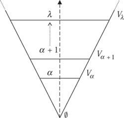
Figure 2 The universe V of all pure sets.
V0 = Ø,
Vα + 1 = P(Vα), the set of all subsets of Vα,
![]() the union of all the Vβ, β < λ, if λ is a limit ordinal.
the union of all the Vβ, β < λ, if λ is a limit ordinal.
The universe of all sets is then the union of all the sets Vα such that α is an ordinal. More concisely,
![]()
3.1 The Axioms of ZFC
The ZFC axioms, stated informally, are the following.
(i) Extensionality. If two sets have the same elements, they are equal.
(ii) Power set. For every set x there is a set P(x) whose elements are all the subsets of x.
(iii) Infinity. There is an infinite set.
(iv) Replacement. If x is a set and ![]() is a function-class1 restricted to x, then there is a set y = {
is a function-class1 restricted to x, then there is a set y = {![]() (u) : u ∈ x}.
(u) : u ∈ x}.
(v) Union. For every set x, there is a set ∪x whose elements are all the elements of the elements of x.
(vi) Regularity. Every set x belongs to Vα, for some ordinal α.
(vii) Axiom of choice (AC). For every set X of pairwise-disjoint nonempty sets there is a set that contains exactly one element from each set in X.
Usually a further axiom appears on this list, called the pairing axiom. It asserts that for any two sets A and B the set {A, B} exists. In particular, {A} exists. Applying the union axiom to the set {A, B} one then gets the union A ∪ B of A and B. But pairing can be derived from the other axioms. Another important axiom that appeared in Zermelo’s original list, one that is both natural and very useful, is the axiom of separation. It states that for every set A and every definable property P, the set of elements of A that have the property P is also a set. But this axiom is a consequence of the axiom of replacement, so there is no need to include it in the list. Using the axiom of separation one can easily prove the existence of the empty set Ø, as well as the intersection A ∩ B and difference A - B of any two sets A and B. The axiom of regularity is also known as the axiom of foundation and it is usually stated as follows: every nonempty set X has an ∈-minimal element, i.e., an element that no element of X belongs to. In the presence of the other axioms the two formulations are equivalent. We chose the formulation in terms of the Vαs to stress the fact that this is a natural axiom based on the construction of the universe of all sets. But it is important to notice that the notions of ordinal and the “cumulative hierarchy of Vαs” need not appear in the formulation of the axioms of ZFC.
The axioms of ZFC lead a kind of double life. On the one hand, they tell us the things we can do with sets. In this sense, ZFC is just like any other collection of axioms for algebraic structures, e.g., the axioms for GROUPS [I.3 §2.1], or FIELDS [I.3 §2.2]: in both cases they give rules for creating new objects from old ones, though there are more rules for sets than there are for group or field elements and they are more complicated. Thus, just as one studies abstract groups, i.e., algebraic structures that satisfy the axioms for groups, so one can study the mathematical structures that satisfy the axioms of ZFC. These are called models of ZFC. Since, for reasons to be explained below, models of ZFC are not easy to come by, one is also interested in models of fragments of ZFC: that is, of axiom systems A that consist of just some of the axioms of ZFC. A model of a fragment A of ZFC is defined to be a pair 〈M, E〉, where M is a nonempty set and E is a binary relation on M, such that all axioms of A are true when the elements of M are interpreted as the sets and E is interpreted as the membership relation. For example, if A includes the union axiom, then for every element x of M there must be an element y of M such that zEy if and only if there exists w such that zEw and wEx. (If we replaced E by ∈ and “element of M” by “set” in the last sentence, then we would recover the usual union axiom.)
The set 〈Vω, ∈〉 is a model of all the axioms of ZFC except infinity, and 〈Vω + ω, ∈〉 is a model of ZFC except replacement. (To see why replacement fails, let x be the set ω and define a function ![]() on x by letting
on x by letting ![]() (n) equal ω + n. The range of
(n) equal ω + n. The range of ![]() belongs to Vω+ω+1 but not to Vω+ω because the ordinal ω + ω does not belong to any set Vω+n and Vω+ω is the union of the sets Vω+n.) For both these models, we took E to be ∈, but one can also look at a completely different relation E on a set M, and see whether it happens to satisfy some of the axioms of ZFC. For example, take the pair 〈
belongs to Vω+ω+1 but not to Vω+ω because the ordinal ω + ω does not belong to any set Vω+n and Vω+ω is the union of the sets Vω+n.) For both these models, we took E to be ∈, but one can also look at a completely different relation E on a set M, and see whether it happens to satisfy some of the axioms of ZFC. For example, take the pair 〈![]() , E〉, where mEn if and only if the mth digit (counting from right to left) in the binary expansion of n is 1. This is a model of ZFC without the axiom of infinity, as the reader may care to check.
, E〉, where mEn if and only if the mth digit (counting from right to left) in the binary expansion of n is 1. This is a model of ZFC without the axiom of infinity, as the reader may care to check.
The other way of thinking of the ZFC axioms is that they tell us how to build up the hierarchy of the Vαs. Axiom (i), the axiom of extensionality, states that a set is something entirely determined by its elements. Axioms (ii)–(v) are tailored to construct V. The power-set axiom is what we use to get from Vα to Vα+1. The axiom of infinity allows the construction to go into the transfinite. Indeed, in the context of the other ZFC axioms, this axiom is equivalent to the assertion that ω exists. The axiom of replacement is used to continue the construction of V at limit stages λ. To see this, consider the function defined by F(x) = y if and only if × is an ordinal and y = Vx. The range of F restricted to λ then consists of all Vβ with β < λ. By the axiom of replacement these sets form a set. Now, by an application of the union axiom to this set one obtains Vλ. Finally, the axiom of regularity states that all sets are obtained in this way: that is, the universe of all sets is precisely V. This rules out pathologies, such as sets that belong to themselves. The point is that for every set X there is a first α such that X ∈ Vα+1. This α is called the rank of X and it marks the stage of the cumulative hierarchy where X was formed. So X could not possibly be an element of itself, since all elements of X must have a rank strictly smaller than the rank of X. The axiom of choice is equivalent, in the context of the other ZFC axioms, to the well-ordering principle.
3.2 Formulas and Models
The ZFC axioms can be formalized using the language of first-order logic for sets. The symbols of first-order logic are variables such as x, y, z, . . . ; the quantifiers “∀” (for all) and “∃” (there exists); the logical connectives “¬” (not), “∧” (and), “∨” (or), “→” (if . . . , then . . .), and “↔” (if and only if); the equality symbol “=”; and parentheses. To make this first-order logic for sets we add one other symbol, “∈,” standing for “is an element of,” and the quantifiers are understood to range over sets. Here is how the axiom of extensionality is expressed in this language:
∀x∀y(∀z(z ∈ x ↔ z ∈ y) → x = y).
This reads as: for every set x and every set y, if every set z belongs to x if and only if it belongs to y (i.e., if x and y have the same elements), then x and y are equal. It is an example of a formula in our language. Formulas can be defined inductively as follows. The atomic formulas are x = y and x ∈ y. Using quantifiers and logical connectives one can build up more complicated formulas using the following rules: if ![]() and
and ![]() are formulas, then so are ¬
are formulas, then so are ¬![]() , (
, (![]() ∧
∧ ![]() ), (
), (![]() ∨
∨ ![]() ), (
), (![]() →
→ ![]() ), (
), (![]() ↔
↔ ![]() ), ∀xϕ and ∃xϕ. Thus, formulas are the formal counterpart of sentences in English (or in any other natural language) that talk only about sets and the membership relation. (For another discussion of formal languages, see LOGIC AND MODEL THEORY [IV.23 §1].)
), ∀xϕ and ∃xϕ. Thus, formulas are the formal counterpart of sentences in English (or in any other natural language) that talk only about sets and the membership relation. (For another discussion of formal languages, see LOGIC AND MODEL THEORY [IV.23 §1].)
Conversely, any formula of the formal language can be interpreted as a sentence (in English) about sets, and it makes sense to ask whether the interpreted sentence is true or not. Usually, by “true” we mean “true in the universe V of all sets,” but it also makes sense to ask about the truth or falsity of a formula in any structure of the form 〈M, E〉, where E is a binary relation on M. For example, the formula ∀x∃y x ∈ y is true in all models 〈M, E〉 of ZFC, while the formula ∃x∀y y ∈ x is false (because of the axiom of regularity). Any formula that can be deduced from the axioms of ZFC is true in all models of ZFC.
Once we have defined what a formula is, we are in a position to make many statements precise that would otherwise not be. For example, the axiom of replacement involves the notion of a function-class. To make proper sense of it one formulates it in terms of first-order formulas. For example, the operation that takes each set a to the singleton {a} is definable, and this depends on the fact that the statement y = {x} can be expressed by the formula ∀z(z ∈ y ↔ z = x). It is not a function, since it is defined on all sets, and the universe of all sets is not a set. This is why we use the different phrase “function-class.” In addition, we sometimes allow parameters in our definitions of function-classes. For example, the function-class that, for a fixed set b, takes each set a to the set a ∩ b is defined by the formula ∀z(z ∈ y ↔ z ∈ x ∧ z ∈ b), which depends on the set b: we call b a parameter and we say that the function-class is definable with parameters. More generally, a function-class is a function on sets given by a formula. But the function itself may not exist as a set, since its domain may contain all sets, or all ordinals, etc. Since the axiom of replacement is a statement about all function-classes, it is not in fact a single axiom but rather an “axiom scheme,” consisting of one axiom for each function-class.
An important consequence of the fact that ZFC can be formalized in first-order logic is that it is subject to a remarkable theorem of Löwenheim and Skolem. The Löwenheím–Skolem theorem is a general result about first-order formal languages; in the particular case of ZFC, it says that if ZFC has a model, then it has a countable model. More precisely, given any model M = 〈M, E〉 of ZFC, there is a model N of ZFC contained in M that is countable and that satisfies exactly the same sentences as M. At first, this may seem paradoxical, for how can ZFC have a countable model if one can prove in ZFC that there are uncountable sets? Does the theorem not lead to a contradiction and therefore imply that there are no models of ZFC? Not quite. Suppose that we have a countable model N of ZFC and a set a in N. If we want to show that the statement “a is countable” is true in N, then we must show that in N there is a surjective map from ω to a. But it is possible for such a map to exist in V, or in some model M that is larger than N, without existing in N, because V and M contain more sets, and therefore more functions, than N does. In such a case, a is uncountable from the point of view of N but countable from the point of view of M or V.
Far from presenting a problem, the relativity of certain set-theoretic notions, like being countable or having a certain cardinality, with respect to different models of ZFC is an important phenomenon which, even if a bit disconcerting at first, may be used to great advantage in consistency proofs (see section 5 below).
It is not difficult to see that all the axioms of ZFC are true in V, which is hardly surprising since they were designed for that to happen. But the ZFC axioms may conceivably hold in some smaller universes. That is, there may be some class M properly contained in V, or even some set M, and therefore by the Löwenheim–Skolem theorem also some countable set M, which is a model of ZFC. As we shall see, while the existence of models of ZFC cannot be proved in ZFC, the fact that one can consistently assume that they exist—provided ZFC is consistent, of course—is of the greatest importance for set theory.
4 Set Theory and the Foundation of Mathematics
As we have seen, we can use ZFC to develop the theory of transfinite numbers. But it turns out that all standard mathematical objects may be viewed as sets, and all classical mathematical theorems can be proved from ZFC using the usual logical rules of proof. For example, real numbers can be defined as certain sets of rational numbers, which can be defined as EQUIVALENCE CLASSES [I.2 §2.3] of ordered pairs of integers. The ordered pair (m, n) can be defined as the set {m, {m, n} }, integers can be defined as equivalence classes of ordered pairs of positive integers, and positive integers can be thought of as finite ordinals, which as we have seen can be defined as sets. Tracing back, one finds that a real number can be regarded as a set of sets of sets of sets of sets of sets of finite ordinals. Similarly, all the usual mathematical objects—such as algebraic structures, vector spaces, topological spaces, smooth manifolds, dynamical systems, and so on—can be shown to exist in ZFC. Theorems concerning these objects can be expressed in the formal language of ZFC, as can their proofs. Of course, writing out a complete proof using the formal language would be extremely laborious, and the result would not only be very long but also virtually impossible to understand. It is important, however, to convince oneself that in principle it can be done. It is the fact that all standard mathematics can be formulated and developed within the axiomatic system of ZFC that makes metamathematics possible, that is, the rigorous mathematical study of mathematics itself. For example, it allows us to think about whether a mathematical statement has a proof: once we have rigorous definitions of “mathematical statement” and “proof,” the question of whether a proof exists becomes a mathematical one with a determinate answer.
4.1 Undecidable Statements
In mathematics the truth of a mathematical statement ϕ is established by means of a proof from basic principles or axioms. Similarly, the falsity of ϕ is established by a proof of ¬ϕ. It is tempting to believe that there must always be a proof of either ϕ or ¬ϕ, but in 1931 GÖDEL [VI.92] proved in his famous INCOMPLETENESS THEOREMS [V.15] that this is not the case. The first incompleteness theorem says that in every axiomatic formal system that is consistent and rich enough to develop basic arithmetic there are undecidable statements: that is, statements such that neither they nor their negations are provable in the system. In particular, there are statements of the formal language of set theory that are neither provable nor disprovable from the ZFC axioms, supposing, that is, that ZFC is consistent.
But is ZFC consistent? The statement that asserts the consistency of ZFC, usually written as CON(ZFC), is the translation into the language of set theory of:
0 = 1 is not provable in ZFC.
This statement asserts that the sequence of symbols 0 = 1 is not the last step of any formal proof from ZFC. One can encode a formal proof as a finite sequence of natural numbers that satisfies certain arithmetical properties, and thereby regard the above statement as an arithmetical one. Gödel’s second incompleteness theorem says that in any consistent axiomatic formal system that is rich enough to develop basic arithmetic, the arithmetical statement that asserts the consistency of the system cannot be proved. Thus, if ZFC is consistent, then its consistency can neither be proved nor disproved in ZFC.
ZFC is currently accepted as the standard formal system in which to develop mathematics. Thus, the truth of a mathematical statement is firmly established if its translation into the language of set theory is provable in ZFC. But what about undecidable statements? Since ZFC embodies all standard mathematical methods, the fact that a given mathematical statement ϕ is undecidable in ZFC means that the truth or falsity of ϕ cannot be established by means of usual mathematical practice. If all undecidable statements were like CON(ZFC), this would probably not be a cause of worry, since they seem not to directly affect the kind of mathematical problems that people are usually interested in. But for better or worse this is not so. As we will see, there are many statements of mathematical interest that are undecidable in ZFC.
There is an obvious way of showing that a mathematical statement has a proof: you just find one. But how can it be possible to prove, mathematically, that a given mathematical statement ϕ is undecidable in ZFC? This question has a short but far-reaching answer. If we can find a model M of ZFC in which ϕ is false, then there cannot be a proof of ϕ (because that proof would show that ϕ was true in M). Therefore, if we can find models M and N of ZFC with ϕ true in M and false in N, we can conclude that ϕ is undecidable.
Unfortunately, a consequence of Gödel’s second incompleteness theorem is that it is not possible to prove in ZFC the existence of a model of ZFC. This is because another theorem of Gödel, called the completeness theorem for first-order logic, asserts that ZFC is consistent if and only if it has a model. However, we can get around this difficulty by splitting the proof of the undecidability of ϕ into two relative consistency proofs: the first is a proof that if ZFC is consistent, then so is ZFC plus ϕ; and the second is a proof that if ZFC is consistent, then so is ZFC plus the negation of ϕ. That is, one assumes that there is a model M of ZFC and proves the existence of two models of ZFC: one where ϕ holds, and one where it fails. One can then conclude that either ϕ and its negation are both unprovable in ZFC, or ZFC is inconsistent, in which case everything is provable.
One of the most surprising results of twentieth-century mathematics is that the continuum hypothesis is undecidable in ZFC.
5 The Continuum Hypothesis
Cantor’s continuum hypothesis (CH), first formulated in 1878, states that every infinite set of real numbers is either countable or has the same cardinality as ![]() . In ZFC, since AC implies that every set, and in particular every infinite set of real numbers, can be put into one-to-one and onto correspondence with a cardinal number, one can easily see that CH is equivalent to the assertion that the cardinality of
. In ZFC, since AC implies that every set, and in particular every infinite set of real numbers, can be put into one-to-one and onto correspondence with a cardinal number, one can easily see that CH is equivalent to the assertion that the cardinality of ![]() is ℵ1, or equivalently, that 2ℵ0 = ℵ1, the version of the statement that we mentioned earlier.
is ℵ1, or equivalently, that 2ℵ0 = ℵ1, the version of the statement that we mentioned earlier.
Solving CH was the first problem in Hilbert’s famous list of twenty-three unsolved problems, and has been one of the main driving forces for the development of set theory. In spite of many attempts at proving CH by Cantor himself and by many leading mathematicians of the first third of the twentieth century, no major progress was made until, sixty years after its formulation, Gödel was able to prove its consistency with ZFC.
5.1 The Constructible Universe
In 1938, Gödel found a way to construct, starting with a model M of ZFC, another model of ZFC, contained in M, where CH holds. He thereby proved the relative consistency of CH with ZFC. Gödel’s model is known as the constructible universe and is represented by the letter L. Since M is a model of ZFC, we may view M as the universe V of all sets. Then L is built inside M in a way that is similar to how we built V, but with the following important difference. When we passed from Vα to Vα+1 we took all subsets of Vα, but to go from Lα to Lα+1 one takes only those subsets of Lα that are definable in Lα. That is, Lα+1 consists of all sets of the form {a : a ∈ Lα and ϕ(a) holds in Lα}, where ϕ(x) is a formula of the language of set theory that may mention elements of Lα. If λ is a limit ordinal, then Lλ is just the union of all the Lα, α < λ, and L is the union of all the Lα, α an ordinal. Of course, we can also build L inside V. This is the real L, the universe of all constructible sets.
One important observation is that to build L it is not necessary to use AC, and so we do not require AC to hold in M. But once L is constructed it can be verified that AC holds in L, as do the other axioms of ZFC. The verification of AC is based on the fact that every element of L is defined at some stage α, and so it is uniquely determined by a formula and some ordinals. Therefore, any sensible well-ordering of all the formulas will naturally yield a well-ordering of L, and thus of every set in L. This shows that if ZF (i.e., ZFC minus AC) is consistent, then so is ZFC. In other words, if we add AC to the ZF axioms, then no contradiction is introduced into the system. This is very reassuring, for although AC has many desirable consequences it also has some that at first sight can appear counterintuitive, such as THE BANACH–TARSKI PARADOX [V.3].
That CH holds in L is due to the fact that in L every real number appears at some countable stage of the construction, i.e., in some Lα, where α is countable in L. To prove this, one shows first that every real r belongs to some Lβ that satisfies a finite number of axioms of ZFC that are sufficient to build L, where β is an ordinal that is not necessarily countable. Then, with the help of the Löwenheim–Skolem theorem, one can show that there is a countable subset X of Lβ that contains r and satisfies the same axioms as Lβ. And then one shows that X must be isomorphic to Lα for some countable ordinal α, via an isomorphism that is the identity on r; this finishes the proof that r appears at a countable stage. But since there are only ℵ1 countable ordinals, and Lα is countable for each countable ordinal α, there can be only ℵ1 real numbers.
Since, for each ordinal α, Lα contains only the sets that are strictly necessary, namely those that were explicitly definable in one of the previous stages, L is the smallest possible model of ZFC containing all the ordinals, and in it the cardinality of ![]() is also the smallest possible, namely ℵ1. In fact, in L the generalized continuum hypothesis (GCH) holds: that is, for every ordinal α, 2ℵα has the smallest possible value, namely, ℵα+1.
is also the smallest possible, namely ℵ1. In fact, in L the generalized continuum hypothesis (GCH) holds: that is, for every ordinal α, 2ℵα has the smallest possible value, namely, ℵα+1.
The theory of constructible sets went through an extraordinary development in the hands of Ronald Jensen. He showed that in L a well-known conjecture called Suslin’s hypothesis was false (see section 10 below) and isolated two important combinatorial principles, known as ◊ (diamond) and ![]() (square), that hold in L. These two principles, which will not be defined here, enable us to carry out constructions of uncountable mathematical structures by induction on the ordinals in such a way that the construction does not break down at limit stages. This is extremely useful, because it allows one to prove consistency results without going to the trouble of analyzing constructible sets: if you can deduce a statement ϕ from ◊ or
(square), that hold in L. These two principles, which will not be defined here, enable us to carry out constructions of uncountable mathematical structures by induction on the ordinals in such a way that the construction does not break down at limit stages. This is extremely useful, because it allows one to prove consistency results without going to the trouble of analyzing constructible sets: if you can deduce a statement ϕ from ◊ or ![]() , then it holds in L, since, by Jensen’s results, ◊ and
, then it holds in L, since, by Jensen’s results, ◊ and ![]() hold in L; it follows that ϕ is consistent with ZFC.
hold in L; it follows that ϕ is consistent with ZFC.
There is also an important generalization of the notion of constructibility, called inner model theory. Given any set A it is possible to build the constructible closure of A, which is the smallest model of ZF that contains all ordinals and A. This model, called L(A), is built in the same way as L, but instead of beginning with the empty set one begins with the transitive closure of A, which consists of A, the elements of A, the elements of the elements of A, and so on. Models of this sort are examples of inner models: that is, models of ZF that contain all the ordinals and all the elements of their elements. Especially prominent are the inner models L(r), where r is a real number, and L(![]() ), the constructible closure of the set of real numbers. Also very important are the inner models of large-cardinal axioms, which will be discussed in section 6 below.
), the constructible closure of the set of real numbers. Also very important are the inner models of large-cardinal axioms, which will be discussed in section 6 below.
After the result of Gödel, and given the repeated failed attempts to prove CH in ZFC, the idea started to take shape that maybe it was undecidable. To prove this, it was necessary to find a way to build a model of ZFC in which CH is false. This was finally accomplished twenty-five years later, in 1963, by Paul Cohen, using a revolutionary new technique called forcing.
5.2 Forcing
The forcing technique is an extremely flexible and powerful tool for building models of ZFC. It allows one to construct models with the most diverse properties and with great control over the statements that will hold in the model being constructed. It has made it possible to prove the consistency of many statements with ZFC that were not previously known to be consistent, and this has led to many undecidability results.
In a manner reminiscent of the way one passes from a field K to an algebraic extension K[a], one goes from a model M of ZFC to a forcing extension M[G] that is also a model of ZFC. However, the forcing method is far more complex, both conceptually and technically, involving set-theoretic, combinatorial, topological, logical, and metamathematical aspects.
To give an idea of how it works, let us consider Cohen’s original problem of starting from a model M of ZFC and obtaining from it a model where CH fails. The only thing we know about M is that it is a model of ZFC, and as far as we know CH may hold in it. In fact, for all we know, M might be the constructible universe L: perhaps when we build L inside M we obtain the whole of M. Therefore, when we extend M we shall have to add to it some new real numbers to ensure that in the extension M[G] there will be at least ℵ2 of them. More precisely, we need the model M[G] to satisfy the sentence that says that there are at least ℵ2-many real numbers. However, the “real numbers” in M[G] may not be real numbers in the actual universe V: all that matters is that in M[G] they satisfy sentences that say “I am a real number.” Similarly, the element of M[G] that plays the role of the cardinal ℵ2 need not be the actual cardinal ℵ2 in V.
In order to explain the method, let us consider the simpler problem of adding to M just a single new real number r. To make things even simpler, let us think of r as just the binary representation of a real in [0, 1]. In other words, r is an infinite binary sequence in the real world V.
A first difficulty is that M may already contain all infinite binary sequences, in which case we will not be able to find one to add. However, by the Löwenheim–Skolem theorem, every model M of ZFC has a countable submodel N that satisfies exactly the same sentences of the language of set theory as M. Let us emphasize that N is countable in the real world, that is, in V; so there is, outside N, a function that enumerates all its elements. Nevertheless, N will contain sets x for which the sentence that says “x is uncountable” is true in N. Since M was a model of ZFC, so is N. So, since we really do not care about the size of M, but only that it is a model of ZFC, we may as well assume that M = N, so that M itself is countable. And now, since there are uncountably many infinite binary sequences, there are plenty of them that do not belong to M.
So, can we just pick any one of them and add it to M? Well, no. The problem is that there are some binary sequences that have a great influence on any model that contains them. For example, we can encode any countable ordinal α as a real number as follows. First let f be a bijection from ![]() to α and define a subset A ⊂
to α and define a subset A ⊂ ![]() 2 to be {(m, n) ∈
2 to be {(m, n) ∈ ![]() 2 : f(m) < f(n)}. Now choose a bijection g from
2 : f(m) < f(n)}. Now choose a bijection g from ![]() to
to ![]() 2 and let c(n) = 1 if and only if g(n) ∈ A. If g is sufficiently explicit (as it can easily be chosen to be), then any model M that contains the infinite binary sequence c must contain the ordinal α, since α can be built out of c using the axioms of ZFC.
2 and let c(n) = 1 if and only if g(n) ∈ A. If g is sufficiently explicit (as it can easily be chosen to be), then any model M that contains the infinite binary sequence c must contain the ordinal α, since α can be built out of c using the axioms of ZFC.
To see why this matters, suppose that M is of the form Lα, as constructed in V, where α is a countable ordinal in V. The existence of models of ZFC of this form follows, for instance, from the existence of large cardinals (see section 6 below), so we certainly cannot rule out this possibility. Since we want to build a model M[c] of ZFC that contains a new infinite binary sequence c and all the elements of M, it will have to contain Lα(c), i.e., all sets that can be constructed in fewer than α steps starting with c. But if c is a sequence that encodes α, as above, then M[c] cannot equal Lα(c) and still be a model of ZFC, since this would imply that Lα(c) contained itself. If we try to circumvent the problem by adding more sets to M[c] so that it becomes a model of ZFC, then we may end up with M[c] = Lγ for some ordinal γ greater than α. And this is not good for our purposes since CH holds in all models of ZFC of the form Lγ. The conclusion is that we cannot just pick an arbitrary c that is not in M: we will have to choose it very carefully.
The key idea is that c should be “generic,” meaning that it should have no special property that singles it out. The reason for this is that if, as before, M = Lα, and we want to ensure that M[c] = Lα(c) is still a model of ZFC, then we do not want c to have any special property that would interfere in the construction of M[c] and cause some ZFC axiom not to hold any more. To accomplish this we build c little by little so that it avoids all the special properties that could possibly have any undesirable effect on M[c]. For example, if we do not want c to encode the ordinal α in the manner sketched above, we simply set some c(n) equal to 0 for some n such that g(n) ∈ A.
Of course, if we have built up the first N binary digits of c and ϕ is a property that holds for all real numbers that begin with those N digits, then we cannot avoid ϕ without undoing our previous work. Let us call a property avoidable if every finite binary sequence p can be extended to a finite binary sequence q such that no infinite sequence that extends q has the property. For instance, the property “all terms in the sequence are zero” is avoidable, while the property “there are ten consecutive ones in the sequence” is not avoidable.
A real number c is called generic, or Cohen, over M if it avoids all avoidable properties that can be defined in M, that is, properties that can be defined by means of formulas that may mention sets in M. It is easy to see that c cannot belong to M, since if it did then the property “is equal to c” would be definable in M, and it is certainly avoidable.
Why should a generic real number exist? Once again, we use the fact that M is countable. From this it follows that there are only countably many avoidable properties. If we enumerate them as ![]() 1,
1, ![]() 2, . . . , then we can pick a finite sequence q1 such that no infinite extension of q1 satisfies
2, . . . , then we can pick a finite sequence q1 such that no infinite extension of q1 satisfies ![]() 1. Then we can extend q1 to q2 such that no infinite extension of q2 satisfies
1. Then we can extend q1 to q2 such that no infinite extension of q2 satisfies ![]() 2. Continuing in this way we create an infinite binary sequence c that does not have any of the properties
2. Continuing in this way we create an infinite binary sequence c that does not have any of the properties ![]() i. In other words, it is generic.
i. In other words, it is generic.
Now let M[c] be the set of all sets that can be constructed, using c and the elements of M as parameters, in as many steps as the ordinals of M. For instance, if M were of the form Lα, then M[c] would just be Lα(c) The model M[c] is called a Cohen-generic extension of M.
It turns out that, miraculously, M[c] is a model of ZFC. Moreover, it has the same ordinals as M and, therefore, it is not of the form Lγ, for any ordinal γ. In particular, when we build L inside M[c], c does not belong to it. These statements are by no means easy to prove, but very roughly what Cohen showed was that a formula ![]() is true in M[c] if and only if there is an initial segment p of c that “forces”
is true in M[c] if and only if there is an initial segment p of c that “forces” ![]() to be true. Moreover, the relation “p forces
to be true. Moreover, the relation “p forces ![]() to be true,” which relates finite binary sequences to formulas and is written p ||-
to be true,” which relates finite binary sequences to formulas and is written p ||- ![]() , can be defined in M. Therefore, to know whether a statement
, can be defined in M. Therefore, to know whether a statement ![]() is true in M[c] one just needs to check whether there is an initial segment p of c such that p ||-
is true in M[c] one just needs to check whether there is an initial segment p of c such that p ||- ![]() . In particular, using this result one can prove that M[c] satisfies the ZFC axioms.
. In particular, using this result one can prove that M[c] satisfies the ZFC axioms.
In order to build a model where CH fails, one adds not just one generic real number but ![]() of them, where
of them, where ![]() is the ordinal that plays the role of
is the ordinal that plays the role of ![]() 2 in M. That is, it is the second uncountable cardinal in M. This need not be the real
2 in M. That is, it is the second uncountable cardinal in M. This need not be the real ![]() 2, and indeed it will not be if, for instance, M is of the form Lα for some countable ordinal α in V. Adding
2, and indeed it will not be if, for instance, M is of the form Lα for some countable ordinal α in V. Adding ![]() generic real numbers can be done by finitely approximating any finite number of them while avoiding all avoidable properties they could have. Thus, instead of finite binary sequences we now work with finite sets of finite binary sequences indexed by ordinals less than
generic real numbers can be done by finitely approximating any finite number of them while avoiding all avoidable properties they could have. Thus, instead of finite binary sequences we now work with finite sets of finite binary sequences indexed by ordinals less than ![]() . A generic object will be a sequence (cα : α <
. A generic object will be a sequence (cα : α < ![]() ) of Cohen reals over M, all different, and so CH is false in the generic extension M[(cα : α <
) of Cohen reals over M, all different, and so CH is false in the generic extension M[(cα : α < ![]() )]
)]
However, there is an important point that needs to be addressed. When we add the new real numbers to M, it is important that the ![]() 2 of the new expanded model is the same as
2 of the new expanded model is the same as ![]() . Otherwise, CH might hold in the expanded model and our work would have been wasted. Fortunately, this is true, but again we must use the facts about forcing to prove it.
. Otherwise, CH might hold in the expanded model and our work would have been wasted. Fortunately, this is true, but again we must use the facts about forcing to prove it.
The same kind of forcing argument allows one to construct models where the cardinality of ![]() is
is ![]() 3, or
3, or ![]() 27, or any other cardinal of uncountable cofinality, i.e., any uncountable cardinal that is not the least upper bound of countably many smaller cardinals. The cardinality of the continuum is, therefore, undetermined by ZFC. Furthermore, since CH holds in Gödel’s constructible universe L and fails in the model constructed by Cohen using forcing, it is undecidable in ZFC.
27, or any other cardinal of uncountable cofinality, i.e., any uncountable cardinal that is not the least upper bound of countably many smaller cardinals. The cardinality of the continuum is, therefore, undetermined by ZFC. Furthermore, since CH holds in Gödel’s constructible universe L and fails in the model constructed by Cohen using forcing, it is undecidable in ZFC.
Cohen also used forcing to prove that AC is independent of ZF. Since AC holds in L, this amounted to constructing a model of ZF in which AC was false. He did this by adding a countable collection (cn : n ∈ ![]() ) of generic real numbers to a countable model M of ZF. To see why this works, let N be the smallest submodel of M[(cn : n ∈
) of generic real numbers to a countable model M of ZF. To see why this works, let N be the smallest submodel of M[(cn : n ∈ ![]() )] that contains all the ordinals and the unordered set A = {cn : n ∈
)] that contains all the ordinals and the unordered set A = {cn : n ∈ ![]() }. Thus, N is just L(A), as built inside M[(cn : n ∈
}. Thus, N is just L(A), as built inside M[(cn : n ∈ ![]() )]. One can then show that N is a model of ZF, but that in N there is no well-ordering of A. The reason is that any well-ordering of A would be definable in L(A) with a finite number of ordinals and finitely many elements of A as parameters, and then each one of the cn would in its turn be definable by indicating its ordinal position in the well-ordering. But since the whole sequence of cns is generic over L, no formula can distinguish one of the cns from another unless they appear as parameters in the formula. Since we can choose two different cns that do not appear as parameters in the definition of the well-ordering of A, and that well-ordering distinguishes all the cns from each other, we have a contradiction. Therefore, the set A cannot be well-ordered, so AC does not hold.
)]. One can then show that N is a model of ZF, but that in N there is no well-ordering of A. The reason is that any well-ordering of A would be definable in L(A) with a finite number of ordinals and finitely many elements of A as parameters, and then each one of the cn would in its turn be definable by indicating its ordinal position in the well-ordering. But since the whole sequence of cns is generic over L, no formula can distinguish one of the cns from another unless they appear as parameters in the formula. Since we can choose two different cns that do not appear as parameters in the definition of the well-ordering of A, and that well-ordering distinguishes all the cns from each other, we have a contradiction. Therefore, the set A cannot be well-ordered, so AC does not hold.
Immediately after Cohen’s proof of the independence of AC from ZF and of CH from ZFC, a result for which he got the Fields Medal in 1966, many set theorists started developing the forcing technique in its full generality (notably Azriel Lévy, Dana Scott, Joseph Shoenfield, and Robert Solovay) and began to apply it to other well-known mathematical problems. For instance, Solovay constructed a model of ZF in which every set of real numbers is LEBESGUE MEASURABLE [III.55], thereby showing that AC is necessary for the existence of nonmeasurable sets. He also constructed a model of ZFC where every definable set of real numbers is Lebesgue measurable; therefore, nonmeasurable sets, although they can be proved to exist (see the example in section 6.1 below), cannot be explicitly given; Solovay and Stanley Tennenbaum developed the theory of iterated forcing and used it to prove the consistency of Suslin’s hypothesis (see section 10 below); Adrian Mathias proved the consistency of the infinitary form of RAMSEY’S THEOREM [IV.19 §2.2]; Saharon Shelah proved the undecidability of the Whitehead problem in group theory; and Richard Laver proved the consistency of the Borel conjecture; to cite just a few remarkable examples from the 1970s.
The forcing technique now pervades all of set theory. It continues to be a research area of great interest, very sophisticated from the technical point of view and of great beauty. It keeps producing important results, with applications in many areas of mathematics, such as topology, combinatorics, and analysis. Especially influential has been the development over the last twenty-five years of the theory of proper forcing, introduced by Shelah. Proper forcing has proved very useful in the context of forcing iterations, and in the formulation and study of new forcing axioms, which will be dealt with in section 10, as well as in the analysis of cardinal invariants of the continuum. These are uncountable cardinals associated with various topological or combinatorial properties of the real line that can consistently take different values in different models obtained by forcing. An example of a cardinal invariant is the least number of null sets needed to cover the real line. Another important development has been the use of class forcing by Anthony Dodd and Ronald Jensen for coding the universe into a single real number, which shows that, amazingly, one can always use forcing to turn any model M into a model of the form L(r) for some real number r. A more recent contribution is the invention by W. Hugh Woodin of new powerful forcing notions associated with the theory of large cardinals (see the next section), which have provided new insights into the continuum hypothesis (see the end of section 10).
The large number of independence results obtained by forcing have made very clear that the axioms of ZFC are insufficient to answer many fundamental mathematical questions. Thus, it is desirable to find new axioms that, once added to ZFC, will provide a solution to some of those questions. We shall discuss some candidates in the next few sections.
6 Large Cardinals
As we have already seen, the collection of all ordinal numbers cannot form a set. But if it did, then to that set there would correspond an ordinal number κ. This ordinal would coincide with the κth cardinal ![]() κ, since otherwise
κ, since otherwise ![]() κ would be a larger ordinal. Moreover, Vκ would be a model of ZFC. We cannot prove in ZFC that there is an ordinal κ with these properties, for then we would have proved in ZFC that ZFC has a model, which is impossible by Gödel’s second incompleteness theorem. So, why do we not add to ZFC the axiom that says that there is a cardinal κ such that Vκ is a model of ZFC?
κ would be a larger ordinal. Moreover, Vκ would be a model of ZFC. We cannot prove in ZFC that there is an ordinal κ with these properties, for then we would have proved in ZFC that ZFC has a model, which is impossible by Gödel’s second incompleteness theorem. So, why do we not add to ZFC the axiom that says that there is a cardinal κ such that Vκ is a model of ZFC?
This axiom, with the further requirement that κ be regular, that is, not the limit of fewer than κ smaller cardinals, was proposed in 1930 by SIERPI![]() SKI [VI.77] and TARSKI [VI.87], and it is the first of the large-cardinal axioms. A cardinal κ with those properties is called inaccessible.
SKI [VI.77] and TARSKI [VI.87], and it is the first of the large-cardinal axioms. A cardinal κ with those properties is called inaccessible.
Other notions of large cardinals, which implied inaccessibility, kept appearing during the twentieth century. Some of them originated in generalizations to uncountable sets of the infinite version of Ramsey’s theorem, which states that if each (unordered) pair of elements of ω (i.e., of natural numbers) is painted either red or blue, then there is an infinite subset X of ω such that all pairs of elements of X have the same color. The natural generalization of the theorem to ω1 turns out to be false. However, on the positive side, Paul Erd![]() s and Richard Rado proved that for every cardinal κ > 2
s and Richard Rado proved that for every cardinal κ > 2![]() 0, if each pair of elements of κ is painted either red or blue, then there is a subset X of κ of size ω1 such that all pairs of elements of X have the same color. This is one of the landmark results of the partition calculus, an important area of combinatorial set theory developed mainly by the Hungarian school, led by Erd
0, if each pair of elements of κ is painted either red or blue, then there is a subset X of κ of size ω1 such that all pairs of elements of X have the same color. This is one of the landmark results of the partition calculus, an important area of combinatorial set theory developed mainly by the Hungarian school, led by Erd![]() s and András Hajnal. The problem of whether Ramsey’s theorem can be generalized to some uncountable cardinal leads naturally to cardinals that are called weakly compact. A cardinal κ is weakly compact if it is uncountable and satisfies the strongest possible Ramsey-type theorem: whenever all pairs of elements of κ are painted either red or blue, there is a subset X of κ of size κ such that all pairs of elements of X have the same color. Weakly compact cardinals are inaccessible, so their existence cannot be proved in ZFC. Moreover, it turns out that below the first weakly compact cardinal, assuming it exists, there are many inaccessible cardinals, so the existence of a weakly compact cardinal cannot be proved even if one assumes the existence of inaccessible cardinals.
s and András Hajnal. The problem of whether Ramsey’s theorem can be generalized to some uncountable cardinal leads naturally to cardinals that are called weakly compact. A cardinal κ is weakly compact if it is uncountable and satisfies the strongest possible Ramsey-type theorem: whenever all pairs of elements of κ are painted either red or blue, there is a subset X of κ of size κ such that all pairs of elements of X have the same color. Weakly compact cardinals are inaccessible, so their existence cannot be proved in ZFC. Moreover, it turns out that below the first weakly compact cardinal, assuming it exists, there are many inaccessible cardinals, so the existence of a weakly compact cardinal cannot be proved even if one assumes the existence of inaccessible cardinals.
The most important large cardinals, the measurable cardinals, are much larger than the weakly compact ones, and were discovered in 1930 by Stanislaw Ulam.
6.1 Measurable Cardinals
A set A of real numbers is a BOREL SET [III.55] if it can be obtained in countably many steps starting from the open intervals and applying the two operations of taking complements and countable unions. It is null, or has measure zero, if for every ε > 0 there is a sequence of open intervals I0, I1, I2, . . . such that A ⊆ Un In and Σn |In| < ε. It is Lebesgue measurable if it is almost a Borel set, that is, if it differs from a Borel set by a null set. To each measurable set A corresponds a number μ(A) ∈ [0, ∞], its measure, that is invariant under translation of A and is countably additive, that is, the measure of a countable union of measurable pairwisedisjoint sets is the sum of their measures. Moreover, the measure of an interval is its length. (See MEASURES [III.55] for a fuller discussion of these concepts.)
One can prove in ZFC that there exist non-Lebesguemeasurable sets of real numbers. For example, the following set was discovered in 1905 by Giuseppe Vitali. Define two elements of the closed interval [0, 1] to be equivalent if they differ by a rational, and let A be a subset of [0, 1] that contains precisely one element from each equivalence class. This requires one to make a large number of choices, which can be done by AC. To see that A is not measurable, consider for each rational p the set Ap = {x + p : × ∈ A}. Any two of these sets are disjoint, because of the way we built A. Let B be the union of all Ap over all rational numbers p in the interval [-1, 1]. A cannot have measure zero, for then B itself would have measure zero, and this is impossible because [0, 1] ⊆ B. On the other hand, A cannot have positive measure either, since then B would have infinite measure, and this is impossible because B ⊆ [-1, 2].
Since measurable sets are closed under taking complements and countable unions, all Borel sets are measurable. In 1905 LEBESGUE [VI.72] showed that there are measurable sets that are not Borel. While reading Lebesgue’s work, Mikhail Suslin noticed that Lebesgue had made a mistake in claiming that continuous images of Borel sets are Borel. Indeed, Suslin soon found a counterexample, which led eventually to the discovery of a new natural hierarchy of sets of reals beyond the Borel sets, the so-called projective sets. These are the sets that can be obtained from the Borel sets by taking continuous images and complements (see section 9 below). In 1917 Nikolai Luzin showed that all continuous images of Borel sets, the analytic sets, are also measurable. If a set is measurable, then so is its complement, so all complements of analytic sets, the coanalytic sets, are also Lebesgue measurable. It is therefore natural to ask whether we can continue like this. In particular, are continuous images of coanalytic sets, or Σ![]() sets, as they are known, also measurable? The answer to this question turns out to be undecidable in ZFC: in L there are Σ
sets, as they are known, also measurable? The answer to this question turns out to be undecidable in ZFC: in L there are Σ![]() sets that are not Lebesgue measurable, and with forcing one can construct models where all Σ
sets that are not Lebesgue measurable, and with forcing one can construct models where all Σ![]() sets are measurable.
sets are measurable.
The proof given above of the existence of a non-Lebesgue-measurable set of reals hinges on the fact that Lebesgue measure is translation invariant. In fact, the proof shows that there cannot be any countably additive translation-invariant measure that extends Lebesgue measure and measures all sets of reals. Thus, a natural question, known as the measure problem, is whether, if one drops the requirement of translation invariance, there can exist some countably additive measure that extends Lebesgue measure and measures all sets of reals. If such a measure exists, then the cardinality of the continuum cannot be ![]() 1, nor
1, nor ![]() 2, nor any
2, nor any ![]() n with n < ω, etc. In fact, Ulam proved in 1930 that a positive solution to the measure problem implies that the cardinality of
n with n < ω, etc. In fact, Ulam proved in 1930 that a positive solution to the measure problem implies that the cardinality of ![]() is extremely large: it is greater than or equal to the least uncountable regular cardinal that is a limit of smaller cardinals. He also proved that the existence of a nontrivial countably additive measure on any set implies either a positive solution to the measure problem, or that there exists an uncountable cardinal κ with a (nontrivial) {0, 1}-valued κ-additive measure that measures all its subsets. Such a cardinal is called measurable. If κ is measurable, then it is weakly compact, and therefore inaccessible. In fact, the set of weakly compact cardinals smaller than κ has measure 1, and so κ is itself the κth weakly compact cardinal. It follows that the existence of a measurable cardinal cannot be proved in ZFC, even if one adds the axiom that inaccessible, or weakly compact, cardinals exist (unless, of course, ZFC plus the existence of such cardinals is inconsistent). A complete clarification of the measure problem was finally provided by Solovay, who showed that if the solution is positive, then there is an inner model with a measurable cardinal. Conversely, if there is a measurable cardinal, then one can build a forcing extension where the measure problem has a positive solution.
is extremely large: it is greater than or equal to the least uncountable regular cardinal that is a limit of smaller cardinals. He also proved that the existence of a nontrivial countably additive measure on any set implies either a positive solution to the measure problem, or that there exists an uncountable cardinal κ with a (nontrivial) {0, 1}-valued κ-additive measure that measures all its subsets. Such a cardinal is called measurable. If κ is measurable, then it is weakly compact, and therefore inaccessible. In fact, the set of weakly compact cardinals smaller than κ has measure 1, and so κ is itself the κth weakly compact cardinal. It follows that the existence of a measurable cardinal cannot be proved in ZFC, even if one adds the axiom that inaccessible, or weakly compact, cardinals exist (unless, of course, ZFC plus the existence of such cardinals is inconsistent). A complete clarification of the measure problem was finally provided by Solovay, who showed that if the solution is positive, then there is an inner model with a measurable cardinal. Conversely, if there is a measurable cardinal, then one can build a forcing extension where the measure problem has a positive solution.
An unexpected consequence of the existence of a measurable cardinal is that the universe V cannot be L: that is, there are nonconstructible sets, and even nonconstructible real numbers. In fact, if there is a measurable cardinal, then V is much larger than L. For instance, the first uncountable cardinal, ![]() 1, is an inaccessible cardinal in L.
1, is an inaccessible cardinal in L.
After the invention of forcing and the subsequent avalanche of independence results, the hope arose that axioms asserting the existence of large cardinals, like measurable cardinals, would settle some of the questions that, thanks to the forcing technique, had been proved undecidable in ZFC. It was soon shown, however, by Lévy and Solovay, that large-cardinal axioms could not settle CH, as one could easily use forcing to change the cardinality of the continuum and make CH hold or fail without destroying the large cardinals. But Solovay proved in 1969 that, surprisingly, if there exists a measurable cardinal, then all Σ![]() sets of real numbers are Lebesgue measurable. So, while the axiom that asserts the existence of a measurable cardinal cannot settle the size of the continuum, it has a profound effect on its structure. It is indeed astonishing that measurable cardinals, so far away from the sets of real numbers in the universe V, have such a strong influence on their basic properties. While the relationship between large cardinals and the structure of the continuum is not yet fully understood, great progress has been made in the last thirty years through the work done in descriptive set theory and determinacy, which will be described in sections 8 and 9 below.
sets of real numbers are Lebesgue measurable. So, while the axiom that asserts the existence of a measurable cardinal cannot settle the size of the continuum, it has a profound effect on its structure. It is indeed astonishing that measurable cardinals, so far away from the sets of real numbers in the universe V, have such a strong influence on their basic properties. While the relationship between large cardinals and the structure of the continuum is not yet fully understood, great progress has been made in the last thirty years through the work done in descriptive set theory and determinacy, which will be described in sections 8 and 9 below.
Some of the deepest and most technically difficult work in set theory is currently devoted to the construction and analysis of canonical inner models for large cardinals. These are analogues of L for large cardinals, that is, they are models built in some canonical way that contain all the ordinals and are transitive (i.e., they contain all elements of their elements), and in which certain large cardinals exist. The larger the cardinal, the more difficult it is to build the model. This work is known as the inner model program.
One of the striking consequences of the inner model program is that it provides a way of measuring the consistency strength of virtually any set-theoretic statement ![]() , using large cardinals. That is, there are large-cardinal axioms A1 and A2 such that the consistency of ZFC plus
, using large cardinals. That is, there are large-cardinal axioms A1 and A2 such that the consistency of ZFC plus ![]() implies that of ZFC plus Al and is implied by the consistency of ZFC plus A2. We refer to A1 as a lower bound for the consistency of
implies that of ZFC plus Al and is implied by the consistency of ZFC plus A2. We refer to A1 as a lower bound for the consistency of ![]() and to A2 as an upper bound. In the fortunate cases when the lower and upper bounds coincide, we obtain an exact measure of the consistency strength of
and to A2 as an upper bound. In the fortunate cases when the lower and upper bounds coincide, we obtain an exact measure of the consistency strength of ![]() . An upper bound A2 is usually obtained by forcing over a model of ZFC plus A2, whereas a lower bound A1 is obtained by inner model theory. Earlier in this section we saw that the consistency strength of a positive solution to the measure problem is exactly that of the existence of a measurable cardinal. We shall see another important example in the next section.
. An upper bound A2 is usually obtained by forcing over a model of ZFC plus A2, whereas a lower bound A1 is obtained by inner model theory. Earlier in this section we saw that the consistency strength of a positive solution to the measure problem is exactly that of the existence of a measurable cardinal. We shall see another important example in the next section.
Knowing upper and lower bounds for the consistency strength of set-theoretic statements—or, even better, knowing their exact consistency strength—is extremely useful for comparing them. Indeed, if the lower bound for a sentence ![]() is greater than the upper bound for another sentence ψ, then we can conclude, via Gödel’s incompleteness theorem, that ψ does not imply
is greater than the upper bound for another sentence ψ, then we can conclude, via Gödel’s incompleteness theorem, that ψ does not imply ![]() .
.
7 Cardinal Arithmetic
Beyond the continuum hypothesis, understanding the behavior of the exponential function 2κ for arbitrary infinite cardinals κ has been a motivating force in set theory. Cantor proved that 2κ > κ for all κ, and Dénes König proved that the cofinality of 2κ is always greater than κ: that is, 2κ is not the limit of fewer than κ smaller cardinals. The GCH, which, as we saw, holds in the constructible universe L, states precisely that 2κ has the least possible value, namely, the least cardinal greater than κ, usually denoted by κ+. One might think that, as in the case of 2![]() 0, by forcing it should be possible to build models of ZFC where 2κ takes any prescribed value, subject only to the necessary requirement that its cofinality should be greater than κ. This is true for cardinals κ that are regular, that is, not the limit of fewer than κ smaller cardinals. Indeed, William Easton showed that for any function F on the regular cardinals such that κ ≤ λ implies F(κ) ≤ F(λ) and F(κ) has cofinality greater than κ, there is a forcing extension of L in which 2κ = F(κ), for all regular κ. So, for instance, one can build a model of ZFC where 2
0, by forcing it should be possible to build models of ZFC where 2κ takes any prescribed value, subject only to the necessary requirement that its cofinality should be greater than κ. This is true for cardinals κ that are regular, that is, not the limit of fewer than κ smaller cardinals. Indeed, William Easton showed that for any function F on the regular cardinals such that κ ≤ λ implies F(κ) ≤ F(λ) and F(κ) has cofinality greater than κ, there is a forcing extension of L in which 2κ = F(κ), for all regular κ. So, for instance, one can build a model of ZFC where 2![]() 0 =
0 = ![]() 7, 2
7, 2![]() 1 =
1 = ![]() 20, 2
20, 2![]() 2 =
2 = ![]() 20, 2
20, 2![]() 3 =
3 = ![]() 101, etc. This shows that the behavior of the exponential function for infinite regular cardinals is totally undetermined in ZFC, and anything possible can be attained by forcing.
101, etc. This shows that the behavior of the exponential function for infinite regular cardinals is totally undetermined in ZFC, and anything possible can be attained by forcing.
But how about nonregular cardinals? Nonregular cardinals are called singular. Thus, an infinite cardinal κ is singular if it is the supremum of fewer than κ smaller cardinals. For instance, ![]() ω, being the supremum of the
ω, being the supremum of the ![]() n, n ∈
n, n ∈ ![]() , is the first singular cardinal. Determining the possible values of the exponential function at singular cardinals is a very hard problem that has generated much important research and involves, quite surprisingly, the necessary use of large cardinals.
, is the first singular cardinal. Determining the possible values of the exponential function at singular cardinals is a very hard problem that has generated much important research and involves, quite surprisingly, the necessary use of large cardinals.
Using a supercompact cardinal, which is a measurable cardinal with certain further properties that make it much larger than ordinary measurable cardinals, Matthew Foreman and Woodin built a model of ZFC in which GCH fails everywhere, i.e., 2κ > κ+ for all cardinals κ. But curiously, the value of the exponential function at a singular cardinal of uncountable cofinality is somehow determined by its values at smaller regular cardinals. Indeed, in 1975, Jack Silver proved that if κ is a singular cardinal of uncountable cofinality and 2α = α+ for all α < κ, then 2κ = κ+. That is, if the GCH holds below κ, then it also holds at κ. That this is also the case for singular cardinals of countable cofinality is a consequence of the singular cardinal hypothesis (SCH), a general principle weaker than the GCH that completely determines singular cardinal exponentiation, relative to exponentiation for regular cardinals. A special case of SCH is the following. If 2![]() n <
n < ![]() ω for all finite n, then 2
ω for all finite n, then 2![]() ω =
ω = ![]() ω+1. So, in particular, if the GCH holds below
ω+1. So, in particular, if the GCH holds below ![]() ω, then it must hold at
ω, then it must hold at ![]() ω. Shelah used his powerful “PCF theory” to obtain the unexpected result that if 2
ω. Shelah used his powerful “PCF theory” to obtain the unexpected result that if 2![]() n <
n < ![]() ω for all n, then 2
ω for all n, then 2![]() ω <
ω < ![]() ω4. So, if GCH holds below
ω4. So, if GCH holds below ![]() ω, then there is a bound (in ZFC!) on the possible values of 2
ω, then there is a bound (in ZFC!) on the possible values of 2![]() ω. But can this value actually be greater than the least possible one, namely
ω. But can this value actually be greater than the least possible one, namely ![]() ω+1? In particular, can the GCH first fail at
ω+1? In particular, can the GCH first fail at ![]() ω The answer is yes, but large cardinals are needed. Indeed, on the one hand Menachem Magidor proved the consistency of the first failure of GCH at
ω The answer is yes, but large cardinals are needed. Indeed, on the one hand Menachem Magidor proved the consistency of the first failure of GCH at ![]() ω, assuming the consistency of the existence of a supercompact cardinal. Thus, the existence of a supercompact cardinal is an upper bound for the failure of SCH. On the other hand, using inner model theory, Dodd and Jensen showed that large cardinals are required for this to happen. An exact measure of the consistency strength of the failure of SCH was later established by Moti Gitik.
ω, assuming the consistency of the existence of a supercompact cardinal. Thus, the existence of a supercompact cardinal is an upper bound for the failure of SCH. On the other hand, using inner model theory, Dodd and Jensen showed that large cardinals are required for this to happen. An exact measure of the consistency strength of the failure of SCH was later established by Moti Gitik.
Figure 3 A run of the infinite game associated with a set A ⊆ [0, 1].
8 Determinacy
It turns out that the existence of very large cardinals, such as supercompact cardinals, has a dramatic effect on the properties of sets of real numbers, especially when they can be defined in some simple way. The link between the two appears through the analysis of certain infinite two-player games that are associated with sets of real numbers. Given a subset A of [0, 1], consider the following infinite game associated with A: there are two players, I and II, who alternately choose a number ni that equals either 0 or 1. To begin with, player I plays n0, then player II plays n1, to which I answers by playing n2, and so on. A run of the game is displayed in figure 3. At the end of the run, the players have produced an infinite binary sequence: n0, n1, n2, . . . . This sequence can be regarded as the binary expansion of a real number r in [0, 1]. Player I wins the game if r belongs to A and player II wins otherwise.
For example, if A is the interval [0, ![]() ], then a winning strategy for player I is simply to start by playing 0, whereas if A = [0,
], then a winning strategy for player I is simply to start by playing 0, whereas if A = [0, ![]() ), then player II wins the game by playing 1 in her first move. But for most games, the question of who wins is not decided after any finite number of moves. For instance, if A is the set of rational points of [0, 1], then one can easily see that player II has a strategy for winning the game (for example, whatever player I does, player II will win if she plays 01001000100001 . . .), but she will not win at any finite stage of the run.
), then player II wins the game by playing 1 in her first move. But for most games, the question of who wins is not decided after any finite number of moves. For instance, if A is the set of rational points of [0, 1], then one can easily see that player II has a strategy for winning the game (for example, whatever player I does, player II will win if she plays 01001000100001 . . .), but she will not win at any finite stage of the run.
The game is determined if one of the two players has a winning strategy. Formally, a strategy for player II is a function ƒ that assigns 0 or 1 to each finite binary sequence of odd length. It is a winning strategy if player II always wins the game if she plays ƒ (n0, n1,. . . , n2k) in her kth turn, whatever moves are made by player I. Similarly, one can define a winning strategy for I. We say that the set A is determined if the game associated with A is determined. One might guess that every game is determined, but actually it is quite easy, using AC, to prove the existence of a game that is not determined.
It turns out that the determinacy of the games associated with certain classes of sets of reals implies that all sets in the class have properties similar to those of the Borel sets. For example, the axiom of determinacy (AD), which asserts that all sets of reals are determined, implies that every set of reals is Lebesgue measurable, has the property of Baire (i.e., differs from an open set by a set of first category), and has the perfect set property (i.e., contains a perfect set if it is uncountable). To give the flavor of a typical argument, let us indicate why every set A of reals is Lebesgue measurable.
First, one observes that it is enough to show that if all measurable subsets of A are null, then A itself must be null. And for this one plays, for every ε > 0, the covering game for A and ε. In this game, player I plays so that the sequence a = (n0, n2, n4, . . .) represents an element of A, and player II plays (binary encodings of) finite unions of rational intervals, with measures adding up to at most ε, while attempting to cover a. It can be shown that if every measurable subset of A is null, then player I cannot have a winning strategy. So by AD there must be a winning strategy for II. Using this strategy one can show that the outer measure of A is at most ε. And since this works for all ε > 0, A must be null.
While AD rules out the existence of badly behaved sets of reals, it implies the negation of AC, so AD is inconsistent with ZFC. However, weaker versions of AD are compatible with, and even follow from, ZFC. Indeed, Donald Martin proved in 1975 that ZFC implies that every Borel set is determined. Moreover, if there exists a measurable cardinal, then every analytic set, and therefore also every coanalytic set, is determined. A natural question, therefore, is whether the existence of larger cardinals implies the determinacy of more complex sets such as the Σ![]() sets.
sets.
The intimate connection between large cardinals and the determinacy of simple sets of reals was first made explicit by Leo Harrington, who showed that the determinacy of all analytic sets is in fact equivalent to a large-cardinal principle slightly weaker than the existence of a measurable cardinal. As we shall shortly see, large cardinals imply the determinacy of certain simply definable sets of reals, the so-called projective sets, while the determinacy of those sets implies in turn the existence of the same kind of large cardinals in some inner models.
9 Projective Sets and Descriptive Set Theory
As we have seen, very basic questions about sets of real numbers can be extremely hard to answer. However, it often turns out to be possible to answer them for sets that occur “in nature,” or that can be explicitly described. This raises the hope that one might be able to prove facts about definable sets of reals that cannot be proved for arbitrary sets.
The study of the structure of definable sets of reals is the subject of descriptive set theory. Examples of such sets are the Borel sets, and also the projective sets, which are sets that can be obtained from Borel sets by taking continuous images and complements. An equivalent definition of the projective sets is that they are subsets of ![]() that can be obtained from closed subsets of
that can be obtained from closed subsets of ![]() n by a mixture of projecting to a lower dimension and taking complements. To see how this relates to definability, consider projecting a subset A ⊂
n by a mixture of projecting to a lower dimension and taking complements. To see how this relates to definability, consider projecting a subset A ⊂ ![]() 2 down to the x-axis. The result will be the set of all x such that there exists y with (x,y) ∈ A. Thus, projection corresponds to existential quantification. Taking complements corresponds to negation, so one can combine the two and obtain universal quantification as well. One can therefore think of a projective set as a set that is definable from a closed set.
2 down to the x-axis. The result will be the set of all x such that there exists y with (x,y) ∈ A. Thus, projection corresponds to existential quantification. Taking complements corresponds to negation, so one can combine the two and obtain universal quantification as well. One can therefore think of a projective set as a set that is definable from a closed set.
Since analytic sets are continuous images of Borel sets, they are projective. And so are the complements of the analytic sets, the coanalytic sets, and the continuous images of coanalytic sets, the Σ![]() sets. More complex projective sets are obtained by taking complements of Σ
sets. More complex projective sets are obtained by taking complements of Σ![]() sets, the so-called Π
sets, the so-called Π![]() sets, their continuous images, called Σ
sets, their continuous images, called Σ![]() , etc. The projective sets form a hierarchy of increasing complexity, in accordance with the number of steps (always finite) that are necessary to obtain them from the Borel sets. Many sets of reals that appear naturally in usual mathematical practice are projective. Moreover, the results and techniques of descriptive set theory, although originally developed for the study of sets of reals, also apply to definable sets in any Polish space (a separable and completemetrizable space). These include basic examples such as
, etc. The projective sets form a hierarchy of increasing complexity, in accordance with the number of steps (always finite) that are necessary to obtain them from the Borel sets. Many sets of reals that appear naturally in usual mathematical practice are projective. Moreover, the results and techniques of descriptive set theory, although originally developed for the study of sets of reals, also apply to definable sets in any Polish space (a separable and completemetrizable space). These include basic examples such as ![]() n,
n, ![]() , separable BANACH SPACES [III.62], etc., where projective sets arise in a very natural way. For example, in the space C[0, 1] of continuous real-valued functions on [0, 1] with the sup norm, the set of everywhere differentiable functions is coanalytic, and the set of functions that satisfy the mean value theorem is Π
, separable BANACH SPACES [III.62], etc., where projective sets arise in a very natural way. For example, in the space C[0, 1] of continuous real-valued functions on [0, 1] with the sup norm, the set of everywhere differentiable functions is coanalytic, and the set of functions that satisfy the mean value theorem is Π![]() . Thus, since descriptive set theory deals with rather natural sets in Polish spaces of general mathematical interest, it is not surprising that it has found many applications in other areas of mathematics such as harmonic analysis, group actions, ergodic theory, and dynamical systems.
. Thus, since descriptive set theory deals with rather natural sets in Polish spaces of general mathematical interest, it is not surprising that it has found many applications in other areas of mathematics such as harmonic analysis, group actions, ergodic theory, and dynamical systems.
Classical results of descriptive set theory are that all analytic sets, and hence also all coanalytic sets, are Lebesgue measurable and have the Baire property, and that all uncountable analytic sets contain a perfect set. However, as we have already pointed out, one cannot prove in ZFC that all Σ![]() sets have those properties, since in L there are counterexamples. By contrast, if there exists a measurable cardinal, then they do have them. But what about more complex projective sets?
sets have those properties, since in L there are counterexamples. By contrast, if there exists a measurable cardinal, then they do have them. But what about more complex projective sets?
The theory of projective sets is closely tied to large cardinals. On the one hand, Solovay showed that if the existence of an inaccessible cardinal is consistent, then so is the statement that every projective set of reals is Lebesgue measurable, has the Baire property, etc. On the other hand, Shelah showed, quite unexpectedly, that the inaccessible cardinal is necessary, in the sense that if all Σ![]() sets are Lebesgue measurable, then
sets are Lebesgue measurable, then ![]() 1 is an inaccessible cardinal in L.
1 is an inaccessible cardinal in L.
Nearly all the classical properties of Borel and analytic sets are shared by the projective sets, assuming that they are determined. So since the determinacy of all projective sets cannot be proved in ZFC and since it allows for the extension of the theory of Borel and analytic sets to all projective sets in a very elegant and satisfactory way, it constitutes an excellent candidate for a new set-theoretic axiom. This axiom is known as projective determinacy (PD). It implies, for instance, that every projective set is Lebesgue measurable, has the Baire property, and has the perfect set property. In particular, since every uncountable perfect set has the same cardinality as ![]() , it implies that there is no projective counterexample to CH.
, it implies that there is no projective counterexample to CH.
One of the most remarkable advances in set theory over the last twenty years is the proof that PD follows from the existence of large cardinals. Martin and John Steel proved in 1988 that if there exist infinitely many so-called Woodin cardinals, then PD holds. Woodin cardinals lie between measurable and supercompact in the hierarchy of large cardinals. Subsequently, Woodin showed that, surprisingly, the hypothesis that for each n it is consistent that there exist n Woodin cardinals is necessary in order to obtain the consistency of PD. Thus the existence of infinitely many Woodin cardinals is a sufficient, and essentially necessary, assumption for extending the classical theory of Borel and analytic sets to all projective sets of reals, and more generally to all projective sets in Polish spaces.
In spite of the enormous success of the known large-cardinal axioms, not only in descriptive set theory but also in many other areas of mathematics, their status as true axioms of set theory is still a matter of debate. This is more so in the case of very large cardinals such as the supercompact ones, the reason being that there is as yet no inner model theory available for them, which means that there is not even strong evidence for their consistency. However, it should be noted that, as Harvey Friedman has shown, large cardinals are necessary even for proving quite simple-looking and rather natural statements about finite functions on the integers, which provides evidence for their essential role in even the most basic parts of mathematics. Another shortcoming of the known large-cardinal axioms is that they cannot decide some fundamental questions. The most conspicuous is CH, but there are others.
10 Forcing Axioms
Another old and basic question about the continuum that the known large-cardinal axioms cannot solve is Suslin’s hypothesis (SH). Cantor had proved that every linearly ordered set that is dense (i.e., any two distinct elements have another element in between), complete (i.e., every nonempty subset with an upper bound has a supremum), separable (i.e., contains a dense countable subset), and without endpoints is order-isomorphic to the real line. In 1920 Suslin conjectured that if instead of separability one assumes the weaker countable chain condition, or CCC, which demands that every pairwisedisjoint collection of open intervals should be at most countable, then it must still be isomorphic to ![]() . The importance of SH for the development of set theory is that it led to the discovery of a new class of axioms, the so-called forcing axioms.
. The importance of SH for the development of set theory is that it led to the discovery of a new class of axioms, the so-called forcing axioms.
In 1967, Solovay and Tennenbaum used forcing to construct a model in which SH holds. The idea is to use the forcing to destroy any counterexamples that there might be to SH. But when one does this one may create new ones, and the result is that one needs to force again and again, transfinitely many times. The iteration of forcing is technically cumbersome and difficult to control, for many unwanted things can happen at the limit stages. For instance, ω1 may be “collapsed,” i.e., it may become countable.
Fortunately, these difficulties can be dealt with. In general, a forcing argument involves a partially ordered set. (In the case we looked at earlier, it was the set of all finite binary sequences, with p < q if p was a proper initial segment of q.) If one starts with a model where GCH holds, uses only partial orderings that are CCC—that is, in which every set of incompatible elements is countable—and takes so-called direct limits at the limit stages, then in ω2 steps one can destroy all counterexamples so that SH holds in the final model. On the other hand, Jensen proved in 1968 that a counterexample to SH exists in L, thereby proving the undecidability of SH in ZFC.
From the construction of Solovay and Tennenbaum, Martin isolated a new principle now known as Martin’s axiom (MA), which generalizes the well-known Baire category theorem. The latter states that in every compact Hausdorff topological space, the intersection of a countable collection of dense open sets is nonempty. MA says the following:
In every compact Hausdorff CCC topological space, the intersection of ![]() 1 dense open sets is nonempty.
1 dense open sets is nonempty.
The condition that the space be CCC (i.e., every collection of pairwise-disjoint open sets is countable) is necessary, for without it the statement is false. It is easy to see that MA implies the negation of CH, for if there are only ![]() 1 real numbers, then the intersection of the
1 real numbers, then the intersection of the ![]() 1 dense open sets
1 dense open sets ![]() {r}, as r ranges over all the real numbers, is empty. However, MA does not decide the cardinality of
{r}, as r ranges over all the real numbers, is empty. However, MA does not decide the cardinality of ![]() .
.
MA has been used with great success to solve many questions that are undecidable in ZFC. For example, it implies SH and that every Σ![]() set is Lebesgue measurable. But is MA really an axiom? In what sense, if any, is it a natural, or at least plausible, assumption about sets? Is the fact that it decides many ZFC undecidable questions sufficient for it to be accepted as being on a par with the ZFC axioms or the axioms of large cardinals? We shall come back to this.
set is Lebesgue measurable. But is MA really an axiom? In what sense, if any, is it a natural, or at least plausible, assumption about sets? Is the fact that it decides many ZFC undecidable questions sufficient for it to be accepted as being on a par with the ZFC axioms or the axioms of large cardinals? We shall come back to this.
MA has many different equivalent formulations. The original formulation of Martin was more closely connected with forcing—hence the term forcing axiom. Roughly speaking it said that if you have a CCC partial order, then you can avoid ![]() 1 avoidable properties, and not just countably many. This allows one to prove the existence of generic subsets of the partial order, over models M of size
1 avoidable properties, and not just countably many. This allows one to prove the existence of generic subsets of the partial order, over models M of size ![]() 1.
1.
Stronger forcing axioms can be obtained by expanding the class of partial orderings to which MA applies while keeping the axiom consistent. An important such strengthening is the proper forcing axiom (PFA), which is formulated for partial orderings that are proper. Properness is a property weaker than the CCC that was discovered by Shelah and is particularly useful when working with complicated forcing iterations. The strongest possible forcing axiom of this type was discovered by Foreman, Magidor, and Shelah in 1988. It is called Martin’s maximum (MM) and is consistent with ZFC, assuming the consistency of a supercompact cardinal.
Both MM and PFA have striking consequences. For example, PFA, and therefore also MM, implies the axiom of projective determinacy (PD), the singular cardinal hypothesis (SCH), and that the cardinality of ![]() is
is ![]() 2.
2.
An advantage of forcing axioms is that one can apply them without having to go into the details of forcing, just as ![]() and
and ![]() save one from having to go into the details of constructible sets. A very good example of this is PFA and some combinatorial principles derived from it, like the so-called open coloring axiom, which have been used with great success by Stevo Todorcevic to solve many outstanding problems in general topology and infinite combinatorics.
save one from having to go into the details of constructible sets. A very good example of this is PFA and some combinatorial principles derived from it, like the so-called open coloring axiom, which have been used with great success by Stevo Todorcevic to solve many outstanding problems in general topology and infinite combinatorics.
As we have already pointed out, forcing axioms are not as intuitively evident as the ZFC axioms, or even the axioms of large cardinals, so one can ask to what extent they should be considered as true axioms of set theory rather than just useful principles for showing that certain statements are consistent with ZFC. In the case of MA and some weaker forms of PFA and MM, some justification for their being taken as true axioms is based on the fact that they are equivalent to principles of generic absoluteness. That is, they assert, under certain restrictions that are necessary to avoid inconsistency, that everything that might exist, does exist. More precisely, if some set having certain properties could be forced to exist over V, then a set having the same properties already exists (in V). So, like the axioms of large cardinals, they are maximality principles, i.e., they attempt to make V as large as possible.
For example, MA is equivalent to the assertion that if a set X having some properties that depend exclusively on subsets of ω1 could be forced to exist over V using a CCC partial ordering ![]() , then such an X already exists in V. This characterization of MA in terms of generic absoluteness provides some justification for regarding MA as a true axiom of set theory. The analogous principle of generic absoluteness, but for proper partial orderings instead of CCC, is known as the bounded proper forcing axiom (BPFA). Although weaker than PFA, BPFA is strong enough to decide many questions that the large-cardinal axioms are unable to settle. Most notably, Justin Moore has recently proved, following a series of results by Woodin, David Asperó, and Todorcevic, that BPFA implies that the cardinality of
, then such an X already exists in V. This characterization of MA in terms of generic absoluteness provides some justification for regarding MA as a true axiom of set theory. The analogous principle of generic absoluteness, but for proper partial orderings instead of CCC, is known as the bounded proper forcing axiom (BPFA). Although weaker than PFA, BPFA is strong enough to decide many questions that the large-cardinal axioms are unable to settle. Most notably, Justin Moore has recently proved, following a series of results by Woodin, David Asperó, and Todorcevic, that BPFA implies that the cardinality of ![]() is
is ![]() 2.
2.
To finish, we briefly mention some deep results that establish strong underlying connections between large cardinals, inner models, determinacy, forcing axioms, generic absoluteness, and the continuum. These results hold under the assumption that for every ordinal α there exists a Woodin cardinal greater than α.
The first one, due to Shelah and Woodin, is that the theory of L(![]() ) is generically absolute. That is, all sentences with real numbers as parameters that would hold in the L(
) is generically absolute. That is, all sentences with real numbers as parameters that would hold in the L(![]() ) of any generic extension of V are already true in the real L(
) of any generic extension of V are already true in the real L(![]() ). This kind of generic absoluteness implies that all sets of reals in L(
). This kind of generic absoluteness implies that all sets of reals in L(![]() ), and in particular the projective sets, are Lebesgue measurable, have the Baire property, etc. Furthermore, by refining the Martin-Steel result that large cardinals imply PD, Woodin showed that in L(
), and in particular the projective sets, are Lebesgue measurable, have the Baire property, etc. Furthermore, by refining the Martin-Steel result that large cardinals imply PD, Woodin showed that in L(![]() ) every set of reals is determined.
) every set of reals is determined.
Another result of Woodin is that there is an axiom, which he calls (*), that is intended to play the role for subsets of ω1 that PD plays for sets of natural numbers, in the sense that it decides “practically all” questions about those sets. Of course, no consistent axiom can really decide all questions that refer only to subsets of ω1, since by Gödel’s incompleteness theorem there will always be undecidable arithmetical statements. So, to formulate precisely the notion of deciding practically all questions, Woodin introduces a new logic, called Ω-logic, that strengthens ordinary first-order logic. One of the main features of Ω-logic is that the valid statements in Ω-logic are generically absolute. Under suitable large-cardinal hypotheses, (*) is consistent in Ω- logic and decides in Ω-logic all questions that refer only to subsets of ω1. The main open problem is the Ω-conjecture, whose formulation is quite technical and beyond the scope of this article. If the Ω-conjecture is true, then any axiom compatible with the existence of large cardinals that decides all questions that depend exclusively on subsets of ω1 in Ω-logic must imply the negation of CH. Thus, the theories ZFC plus CH and ZFC plus not-CH are not equally reasonable from the point of view of Ω-logic, since in the presence of large cardinals CH puts an unnecessary limitation on the possibility of settling all natural questions about subsets of ω1.
11 Final Remarks
In this short account of set theory, we have reviewed some of the key developments since its beginnings in the late nineteenth century. What started in the hands of Cantor as a mathematical theory of transfinite numbers has developed to become a general theory of infinite sets and a foundation for mathematics. The fact that it has been possible to unify all of classical mathematics into one single theoretical framework, the ZFC axiom system, is certainly remarkable. But beyond this, and most importantly, the techniques developed by set theory, such as constructibility, forcing, infinite combinatorics, the theory of large cardinals, determinacy, the descriptive theory of definable sets in Polish spaces, etc., have turned it into a discipline of great depth and beauty, with fascinating results that stimulate and challenge our imagination, and with numerous applications in areas such as algebra, topology, real and complex analysis, functional analysis, and measure theory. In the twenty-first century, the ideas and techniques generated within set theory will surely continue to contribute to the solution of outstanding mathematical problems, old as well as new, and will help mathematicians gain an ever deeper insight into the complexities and vastness of the mathematical universe.
Further Reading
Foreman, M., and A. Kanamori, eds. 2008. Handbook of Set Theory. New York: Springer.
Friedman, S. D. 2000. Fine Structure and Class Forcing. De Gruyter Series in Logic and Its Applications, volume 3. Berlin: Walter de Gruyter.
Hrbacek, K., and T. Jech. 1999. Introduction to Set Theory, 3rd edn., revised and expanded. New York: Marcel Dekker.
Jech, T. 2003. Set Theory, 3rd edn. New York: Springer.
Kanamori, A. 2003. The Higher Infinite, 2nd edn. Springer
Monographs in Mathematics. New York: Springer.
Kechris, A. S. 1995. Classical Descriptive Set Theory. Graduate Texts in Mathematics. New York: Springer.
Kunen, K. 1980. Set Theory: An Introduction to Independence Proofs. Amsterdam: North-Holland.
Shelah, S. 1998. Proper and Improper Forcing, 2nd edn. New York: Springer.
Woodin, W. H. 1999. The Axiom of Determinacy, Forcing Axioms, and the Nonstationary Ideal. De Gruyter Series in Logic and Its Applications, volume 1. Berlin: Walter de Gruyter.
Zeman, M. 2001. Inner Models and Large Cardinals. De Gruyter Series in Logic and Its Applications, volume 5. Berlin: Walter de Gruyter.
1. A function-class can be thought of as a function that is given as a definition rather than an object that has to exist as a set. The concept will be made precise in section 3.2.