
IV.4 Algebraic Geometry
János Kollár
1 Introduction
Succinctly put, algebraic geometry is the study of geometry using polynomials and the investigation of polynomials using geometry.
Many of us were taught the beginnings of algebraic geometry in high school, under the name “analytic geometry.” When we say that y = mx + b is the equation of a line L, or that x2 + y2 = r2 describes a circle C of radius r, we establish a basic connection between geometry and algebra.
If we want to find the points where the line L and the circle C intersect, we just substitute mx + b for y in the circle equation to get x2 + (mx + b)2 = r2 and solve the resulting quadratic equation to obtain the x coordinates of the two intersection points.
This simple example encapsulates the method of algebraic geometry: a geometric problem is translated into algebra, where it is readily solvable; conversely, we get insight into algebra problems by using geometry. It is hard to guess the solutions of systems of polynomial equations, but once a corresponding geometric picture is drawn, we start to have a qualitative understanding of them. The precise quantitative answer is then provided by algebra.
2 Polynomials and Their Geometry
Polynomials are the expressions one can put together from variables and numbers by addition and multiplication. The most familiar are one-variable polynomials such as x3 - x + 4, but we can use two or three variables to get, for instance, 2x5 - 3xy2 + y3 (which has degree 5 in two variables) or x5 - y7 + x2 z8 - xyz + 1 (which has degree 10 in three variables). In general, one can use n variables, in which case they are frequently denoted by x1, x2, . . . , xn, and we write f(x1, . . . , xn), f(x) or simply f to denote an unspecified polynomial.
Polynomials are the only functions that computers can work with. (Although your pocket calculator is likely to have a button for logarithms, it is secretly computing a polynomial whose value at a number b agrees with log b up to many decimal places.)
We can slightly rewrite the equations we gave earlier for the line L and the circle C: as y - mx - b = 0 and x2 + y2 - r2 = 0. We can then describe L and C as zero sets: L is the zero set of y - mx - b (that is, the set of all points (x, y) such that y - mx - b = 0) and C is the zero set of x2 + y2 - r2.
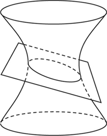
Figure 1 A hyperboloid intersecting a plane.
Similarly, the zero set of 2x2 + 3y2 - z2 - 7 in 3-space is a hyperboloid, the zero set of z - x - y in 3-space is a plane, and the common zero set of these two equations in 3-space is the intersection of the hyperboloid and the plane, which is an ellipse (see figure 1).
The set of common zeros of a system of polynomial equations in any number of variables is called an algebraic set. These are the basic objects of algebraic geometry.
Most people feel that geometry ends in 3-space. Very few have a feeling for 4-space, also called space-time, and 5-space is by and large inconceivable to almost everyone. So what is the meaning of geometry in many variables?
Algebra comes to our rescue here. While I have great difficulty visualizing what a four-dimensional sphere of radius r in 5-space should be, I can easily write down its equation,
![]()
and work with it. This equation is also something a computer can handle, which is immensely useful in applications.
I will, nonetheless, stick to two or three variables for the rest of this article. This is where all geometry starts and there are plenty of interesting questions and results.
The importance of algebraic geometry derives from the fact that significant interactions between algebra and geometry happen very frequently. Let us look at two examples, just for illustration.
3 Most Shapes Are Algebraic
Shapes that occur frequently enough to have their own name, for instance, lines, planes, circles, ellipses, hyperbolas, parabolas, hyperboloids, paraboloids, ellipsoids, are almost all algebraic. Even the more esoteric conchoid (or shell curve) of Dürer, the trident of NEWTON [VI.14], and the folium of Kepler are algebraic.
Some shapes cannot be described by polynomial equations, but they can be described by polynomial inequalities. For instance, the inequalities 0 ≤ x ≤ a and 0 ≤ y ≤ b together describe a rectangle with side lengths a, b. Shapes described by polynomial inequalities are called semialgebraic, and every polyhedron is semialgebraic.
Not everything is an algebraic set, though. Look, for example, at the graph of the sine function y = sinx. This crosses the x-axis infinitely many times (at multiples of π). If f(x) is any polynomial, then it has at most as many roots as its degree, so y = f(x) will never look like y = sinx.
We can, however, get very close to sinx with a polynomial if we concentrate on values of x that are not too large. For instance, the degree-7 Taylor polynomial
![]()
differs from sinx by an error of at most 0.1 for -π < x < π. This is a very special case of a basic theorem of Nash that says that every “reasonable” geometric shape is algebraic if we ignore what happens very far from the origin. So, what is reasonable? Certainly not everything. Fractals seem profoundly nonalgebraic. The nicest shapes are MANIFOLDS [I.3 §6.9], and all of these can be described by polynomials.
Nash’s theorem. Let M be any manifold in ![]() . Fix any large number R. Then there is a polynomial f whose zero set is as close to M as we want, at least inside a ball of radius R around the origin.
. Fix any large number R. Then there is a polynomial f whose zero set is as close to M as we want, at least inside a ball of radius R around the origin.
4 Codes and Finite Geometries
Consider the equation x2 + y2 = z2, which describes a double cone in 3-space (see figure 4). If we confine ourselves to natural numbers, then the solutions of x2 + y2 = z2 are the Pythagorean triples, corresponding to right-angled triangles where all sides have integer lengths, of which the two best-known examples are (3, 4, 5) and (5, 12, 13).
Let us now look at the same equation, but declare that we care only about the parities of the two sides (that is, whether they are even or odd). For instance, 32 + 152 and 42 are both even, so we say that 32 + 152 = 42 (mod 2). The parities of x2 + y2 and of z2 depend only on those of x, y, and z, so we can pretend that x, y, and z are all either 0 (the even case) or 1 (the odd case). Our equation modulo 2 therefore has four solutions:
000, 011, 101, 110.
These look like code words in a computer message. It was quite a surprise when it was discovered that using polynomials and their solutions modulo 2 is a great—probably the best—way of constructing ERROR- CORRECTING CODES [VII.6 §§3-5].
There is something very substantial and new happening here. Let us think for a moment about what 3-space is for us. For many it is an amorphous everything, but for algebraic geometers (with DESCARTES [VI.11] as our ancestor) it is simply a collection of points described by three numbers, the x, y, and z coordinates. Let us make a jump here, and declare that “3-space modulo 2” is the collection of all “points” given by three coordinates modulo 2. Four of these are listed above, and there are four more. The beauty of algebra is that suddenly we can talk about lines, planes, spheres, cones in this “3-space having only eight points.”
We do not need to stop here, and one can work modulo any integer. For example, working modulo 7, we have 0, 1, 2, 3, 4, 5, 6 as possible coordinates, and so “3-space modulo 7” has 73 = 343 points.
Talking about geometry in these spaces is very intriguing, but also technically difficult. Its great reward is that one can view this process as a “discretization” of ordinary space. Working modulo n for large n (especially when n is a prime number) gets very close to the usual geometry.
This approach is especially fruitful in number-theoretic questions. It was, for instance, instrumental in Wiles’s proof of Fermat’s last theorem.
For more on these topics, see ARITHMETIC GEOMETRY [IV.5].
5 Snapshots of Polynomials
Consider the equation x2 + y2 = R. If R > 0, then the real solutions form a circle of radius ![]() ; if R = 0, we get only the origin; and if R < 0, we get the empty set. Thus, if R > 0, then the geometry of the solution set determines what R is, but otherwise it does not. We can of course look at complex solutions, and the complex solutions always determine R. (For instance, the intersection points with the x-axis are (±
; if R = 0, we get only the origin; and if R < 0, we get the empty set. Thus, if R > 0, then the geometry of the solution set determines what R is, but otherwise it does not. We can of course look at complex solutions, and the complex solutions always determine R. (For instance, the intersection points with the x-axis are (±![]() , 0).)
, 0).)
If R is a rational number, we can ask about rational solutions of x2 + y2 = R, and if R is an integer, we can also look for solutions in the “plane modulo m” for any m.
One can even look for solutions where x = x(t), y = y(t) are themselves polynomials in a variable t. (Most generally, we can ask for solutions where x, y are elements of any ring containing the number R.)
To my mind, the polynomial is the central object, and each time we look at solution sets we are taking a “snapshot” of the polynomial. Some snapshots are good (like the above real snapshot for R > 0) and some are bad (like the above real snapshot for R < 0).
How good can snapshots be? Can we determine a polynomial from its snapshots?
One frequently talks about “the” equation of a hyperbola, but “an” equation would be more correct. Indeed, the hyperbola x2 - y2 - R = 0 can also be given by an equation cx2 - cy2 - cR = 0, for any c ≠ 0. We can also use the equation (x2 - y2 - R)2 = 0, which we may well not recognize in its expanded form. Higher powers can also be used. What about the equation f(x, y) = (x2 - y2 - R)(x2 + y2 + R2) = 0? If we look only at real solutions, this is still just the hyperbola since x2 + y2 + R2 is always positive for x, y real. However, as with one-variable polynomials, one should look at all complex roots to understand everything. Then we see that f(![]() R, 0) = 0, but the complex point (
R, 0) = 0, but the complex point (![]() R, 0) is not on the hyperbola x2 - y2 - R = 0. In general, as long as R ≠ 0, we get that if f is a polynomial that has exactly the same complex roots as x2 - y2 - R, then f(x, y) = c(x2 - y2 - R)m for some m and c ≠ 0.
R, 0) is not on the hyperbola x2 - y2 - R = 0. In general, as long as R ≠ 0, we get that if f is a polynomial that has exactly the same complex roots as x2 - y2 - R, then f(x, y) = c(x2 - y2 - R)m for some m and c ≠ 0.
Why is the R = 0 case different? The reason is that for R ≠ 0 the polynomial x2 - y2 - R is irreducible (that is, it cannot be written as the product of other polynomials), while x2 - y2 = (x + y)(x - y) is reducible with irreducible factors x + y and x - y. In the latter case one gets that if g(x, y) is a polynomial that has exactly the same complex roots as x2 - y2>, then f = c · (x + y)m(x - y)n for some m, n and c ≠ 0.
The analogous question for systems of equations is answered by the fundamental theorem of algebraic geometry. It is sometimes called Hilbert’s theorem on the zeros, but its German name is used most of the time. For simplicity, we state only the case of one equation.
Hilbert’s Nullstellensatz. Two complex polynomials f and g have the same complex solutions if and only if they have the same irreducible factors.
We can do even better for polynomials with integer coefficients. For instance, x2 - y2 - 1 = 0 and 2(x2 - y2 - 1) = 0 have the same solutions over the real or complex numbers, and the same solutions modulo p for any odd prime p, but they have different solutions modulo 2. The general result in this case is easy and simple.
Arithmetic Nullstellensatz. Two polynomials with integer coefficients f and g have the same solutions modulo m for every m if and only if f = ±g.
6 Bézοut’s Theorem and Intersection Theory
If h(x) is a polynomial of degree n, then it has n complex roots, at least when they are counted with multiplicity. What happens with a system f(x, y) = g(x, y) = 0? Geometrically we see two curves in the plane, so we expect that there will typically be finitely many intersection points.
If f, g are both linear, we have two lines in the plane. These usually intersect in a single point, but they can be parallel and they can coincide. The first case leads to the classical declaration that “parallel lines meet at infinity” and the definition of projective planes and PROJECTIVE SPACES [III.72]. (The introduction of projective spaces and the corresponding projective varieties is a key step in algebraic geometry. It is somewhat technical so we shall skip it here, but it is indispensable even at the most basic level.)
Next, consider two polynomials of degree 2, that is, two plane conics. Two smooth conics usually intersect in at most four points (just try this by drawing two ellipses). There are also some rather degenerate cases. Two conics may coincide, or, if they are both reducible, they can have a common line. In any case, we are ready to formulate a basic result, dating back to 1779.
Bézout’s theorem. Let f1 (x), . . . , fn(x) be n polynomials in n variables, and for each i let di be the degree of fi. Then either
(i) the equation(s) f1(x) = . . . = fn(x) = 0 have at most d1 d2 . . . dn solutions; or
(ii) the fi vanish identically on an algebraic curve C, and so there is a continuous family of solutions.
As an example, the second alternative happens for the system of equations xz - y2 = y3 - z2 = x3 - z = 0, which has (t, t2, t3) as a solution for any t. This case is actually quite rare. If we pick the coefficients of the polynomials fi randomly, then the first alternative happens with probability 1.
Ideally, we would like to make the stronger claim that if the first alternative happens, then there are exactly d1 d2 . . . dn solutions, but counted “with multiplicity.” This actually works, and gives us our first example of an extremely useful feature of algebraic geometry. Even in very degenerate situations it is possible to define and count the multiplicities easily. This is frequently of great help since the typical (or “generic”) cases are usually very hard to compute. To get around this problem, we can sometimes find a special, degenerate case where we know that the answer will be the same, but the computations are much easier.
There are two ways to think about multiplicity: one algebraic and one geometric. The algebraic definition is computationally very efficient, but somewhat technical. The geometric interpretation is easier to explain, so that is the one we shall give here, but it would be hard to compute with in practice.
If x = p is an isolated solution of the equations f1(x) = . . . = fn(x) = 0 with multiplicity m, then the perturbed system
f1(x) + ∈1 = . . . = fn(x) + ∈n = 0
has exactly m solutions near x = p for almost all small values of the ∈i.
Intersection theory is the branch of algebraic geometry that deals with generalizations of Bézout’s theorem. Above, we looked at intersections of hypersurfaces—that is, of zero sets of single polynomials—but we may wish to look at intersections of more general algebraic sets. Also, even when the second alternative holds, we may want to count the number of isolated intersection points; this can be very tricky but also very useful.
7 Varieties, Schemes, Orbifolds, and Stacks
Consider the system xz = yz = 0 in 3-space. It consists of two pieces, the z = 0 plane and the x = y = 0 line. It is easy to see that neither the plane nor the line can be written as the union of algebraic sets (except by nitpickers who point out that the line is the union of the line itself and of any point on the line). In general, any algebraic set can be written in exactly one way as the union of smaller algebraic sets that in turn cannot be decomposed further. These basic building blocks are called irreducible algebraic sets or algebraic varieties.

Figure 2 A smooth cubic: y2 = x3 - x.
Sometimes this is not exactly what one would naively expect. For instance, the curve in figure 2 has two connected components. The two parts are, however, not algebraic sets.
An explanation is provided by looking at the complex solutions of this equation. We shall see later that these form a connected set, namely a torus (with a missing point at infinity) We see two components when we look at the real solutions because we are taking a cross-section of this torus.
In general, the zero set f = 0 is irreducible as an algebraic set if and only if f is irreducible as a polynomial (or if it is the power of an irreducible polynomial). The implication in one direction is easy to see: if f = gh, then the zero set of f is the union of the zero set of g and of the zero set of h.
For many questions, keeping track only of the zero set is not enough. For instance, look at the polynomial f = x2 (x - 1)(x -2)3. It has degree 6 and three roots at x = 0, 1, 2. These roots behave differently, however, and one usually says that f has a double root at x = 0 and a triple root at x = 2. If we perturb f by adding a small number ∈ to it, then the perturbed equation f(x) + ∈ = 0 has two (complex) solutions near 0, one solution near 1 and three (complex) solutions near 2. Thus, these multiplicities carry important geometric meaning about the perturbation of the equation.
Similarly, it is natural to say that while x2 y = 0 and xy3 = 0 define the same algebraic set (consisting of the two axes), the first “assigns multiplicity 2” to the y-axis and the other “assigns multiplicity 3” to the x-axis.
More complicated things can happen for systems of equations. Consider the systems x = y2 = 0 and x3 = y = 0 in 3-space. Both define the z-axis and it is reasonable to say that the first does so with multiplicity 2, the second with multiplicity 3. There is, however, a further difference. In the first case the multiplicity seems to “go in the y-direction” and in the second case it seems to go in the x-direction. We can also look at other systems, like x - cy = y3 = 0, if we want to see more complicated behavior.
Roughly speaking, a scheme is an algebraic set where we also keep track of the multiplicities and of the directions they occur in.
Consider the xy-plane and consider the map that reflects across the origin. Thus a point (x, y) is mapped to (-x, -y). Let us try to glue each point (x, y) to its image (-x, -y). What do we get? The right half-plane x ≥ 0 is mapped to the left half-plane x ≤ 0, so it is enough to work out what happens with the right half- plane. The positive y-axis is glued to the negative y- axis, and the resulting surface is a dunce cap (but less pointy).
Algebraically, it is one half of the cone z2 = x2 + y2. This cone looks nice and smooth except at the vertex. There it is more complicated, but the above construction shows that it can be obtained from a plane by a reflection across a point. More generally, suppose we take the n-dimensional space ![]() and finitely many symmetries of it. If we glue together points that move into each other, we again get an algebraic variety, most of whose points are smooth, but some of which are more complicated. A variety made up of pieces like these is called an orbifold. (When this is defined more precisely, we also keep track of which symmetries have been used.) In practice, such varieties occur frequently; that is why they deserve a separate name.
and finitely many symmetries of it. If we glue together points that move into each other, we again get an algebraic variety, most of whose points are smooth, but some of which are more complicated. A variety made up of pieces like these is called an orbifold. (When this is defined more precisely, we also keep track of which symmetries have been used.) In practice, such varieties occur frequently; that is why they deserve a separate name.
Finally, if we marry a scheme to an orbifold, the outcome is a stack. The study of stacks is strongly recommended to people who would have been flagellants in earlier times.
8 Curves, Surfaces, Threefolds
As with any geometric object, one of the simplest questions one can ask about a variety is: what is its dimension? As expected, a curve in the plane has dimension 1, and a surface in 3-space has dimension 2. This seems quite simple until one writes down examples like S = (x4 + y4 + z4 = 0), which is only the origin in ![]() . This example is, nonetheless, still two dimensional: the explanation is that we were looking at the wrong snapshot. Using complex numbers we can solve the equation as
. This example is, nonetheless, still two dimensional: the explanation is that we were looking at the wrong snapshot. Using complex numbers we can solve the equation as ![]() so the complex solutions of x4 + y4 + z4 = 0 can be described by two independent variables x, y and a dependent variable z. Thus, it is quite reasonable to say that S is two dimensional.
so the complex solutions of x4 + y4 + z4 = 0 can be described by two independent variables x, y and a dependent variable z. Thus, it is quite reasonable to say that S is two dimensional.
This idea works more generally. If X is any variety in some complex space ![]() , then choose a random set of n independent directions to serve as a basis, or coordinate system, for
, then choose a random set of n independent directions to serve as a basis, or coordinate system, for ![]() , and hence for X. With probability 1 (i.e., except in degenerate cases) one finds that there is some d such that the first d coordinates of a point x in X can vary independently, while the rest depend on them. This number d depends on X only and is called the dimension (or, to be precise, the algebraic dimension) of X.
, and hence for X. With probability 1 (i.e., except in degenerate cases) one finds that there is some d such that the first d coordinates of a point x in X can vary independently, while the rest depend on them. This number d depends on X only and is called the dimension (or, to be precise, the algebraic dimension) of X.
If X is a variety and f is a polynomial, then the intersection X ∩(f = 0) has dimension one less than dim X (unless f vanishes identically on X or never takes the value zero on X).
If X is a subset of ![]() defined by real equations, and if it is smooth (see the next section for a discussion of smoothness), then its TOPOLOGICAL DIMENSION [III.17] is the same as its algebraic dimension.
defined by real equations, and if it is smooth (see the next section for a discussion of smoothness), then its TOPOLOGICAL DIMENSION [III.17] is the same as its algebraic dimension.
For complex varieties, the topological dimension is twice the algebraic dimension. Thus, for an algebraic geometer,![]() has dimension n. In particular, for us
has dimension n. In particular, for us ![]() is the “complex line,” whereas everybody else calls this the “complex plane.” Our “complex plane” is, of course,
is the “complex line,” whereas everybody else calls this the “complex plane.” Our “complex plane” is, of course, ![]() .
.
A variety of dimension 1 is called a curve. A surface is a variety of dimension 2, and a threefold is a variety of dimension 3.
The theory of algebraic curves is a very well developed and beautiful subject. We shall see later how one can start to get an overview of all algebraic curves. Surfaces have been intensively studied for the last century, and now we have reached a reasonably complete understanding of them. This is a much more complicated theory than for curves. Still very little is known for varieties of dimension 3 and up. At least conjecturally, all these dimensions behave in roughly the same way. Despite some progress, especially in dimension 3, many questions are wide open.
9 Singularities and Their Resolutions
If we look at the simplest examples of algebraic curves in figure 3, we see that most points of a curve are smooth, but that there may be a finite set of more complicated singular points. Let us compare these with the curve in figure 2.
All three curves pass through the origin, since their equation has no constant term. The equation of figure 2 has a linear term and the curve looks nice and smooth at the origin, whereas the equations of figure 3 contain no linear term and the curves are more complicated at the origin. This is not an accident. For small values of x, the higher powers x2, x3, . . . are much smaller than x in absolute value, so near the origin the linear terms dominate. If we have only linear terms ax + by = 0, we get a line through the origin, and an algebraic curve ax + by + cx2 + gxy + ey2 + . . . = 0 is close to the line ax + by = 0, at least for very small values of x and y.

Figure 3 Singular cubics: (a) y2 = x3 + x2 and (b) y2 = x3.
The study of a curve near another point with coordinates (p, q) can be reduced to the case (p, q) = (0, 0) via the coordinate change (x,y) ![]() (x - p, y - q).
(x - p, y - q).
In general, if f(0) = 0 and f has a (nonzero) linear term L(f), the hypersurface f = 0 is very close to the hyperplane L(f) = 0. This is the so-called implicit function theorem. Such points are called smooth. Points that are not smooth are called singular. One can easily show that the singular points of X form an algebraic set, defined by the vanishing of all partial derivatives ∂f/∂xi. A random hypersurface will, with probability 1, be smooth, but there are many singular hypersurfaces as well.
The smooth and singular points of an arbitrary variety of dimension d can be defined analogously by comparing X with d-dimensional linear subspaces.
Singularities also occur in other geometric fields, such as topology and differential geometry, but by and large these fields shy away from their study (with the notable exception of catastrophe theory). By contrast, algebraic geometry provides very powerful tools for their investigation.
Let us start with singularities of hypersurfaces, or equivalently with critical points of functions. When thinking about these it is natural to work not just with polynomials but with more general power series, that is, functions f(x1, . . . , xn) that can be written as “polynomials of infinite degree.” For simplicity of notation we shall assume that f(0) = 0. Two functions f, g are considered to be equivalent if there is a coordinate change xi ![]()
![]() i(x), where each
i(x), where each ![]() i is given by a power series, such that f(
i is given by a power series, such that f(![]() 1(x), . . . ,
1(x), . . . , ![]() n(x)) = g(x).
n(x)) = g(x).
In the one-variable case, any f can be written as
f = xm(am + am+1 x + . . .),
where am ≠ 0. The (inverse of the) substitution
![]()
then shows that f is equivalent to xm. The functions xm are inequivalent for different values of m, so in this particular case the lowest-degree monomial occurring in f determines f up to equivalence. (Note that even if f is a polynomial, the above change of variable involves an infinite power series: it is because we cannot invert polynomials, even locally, that it is more convenient to consider general power series.)
In general, the lowest-degree terms of a power series do not determine the singularity, but taking more terms is usually enough to do so, because of the following result.
Algebraization of analytic singularities. Given a power series f, let f≤N denote the polynomial obtained from f by deleting all monomials of degree greater than N. If 0 is an isolated singular point of the hypersurface (f = 0), then f is equivalent to f≤N for sufficiently large N.
To see an example of a nonisolated singularity at 0, take

It has singular points not just at 0, but everywhere along the curve y + (x/(1 - x)) = z = 0. On the other hand, one can easily check that all truncations g≤N do have an isolated singular point at 0.
If we have two power series, f and g, we can view functions of the form f + ∈g as perturbations of f. A very fruitful question of singularity theory asks: what can we say about the perturbations of a given polynomial or power series f ?
For instance, in the one-variable case, the polynomial xm can be perturbed as xm + ∈xr, which is equivalent to xr if r < m. Every perturbation contains xm, so if r > m, then no perturbation of xm will be equivalent to xr (because near the origin xm will be much larger than xr). Hence, up to equivalence, the set of all possible perturbations of xm is {xr : r ≤ m}.
On the other hand, it is not hard to see that for any given ∈, there are only twenty-four different values of η for which the polynomials xy(x2 - y2) + ∈y2(x2 - y2) and xy (x2 - y2) + ηy2 (x2 - y2) are equivalent. (Indeed, both polynomials describe four lines through the origin. The first one gives the lines y = 0, x = y, x = -y, and x = -∈y, and the second gives the same lines except that η replaces ∈. The linear part of any supposed equivalence gives a linear transformation mapping the first set of four lines to the second. There are twenty-four ways to assign which line goes to which line.) Thus xy(x2 - y2) has a continuous family of inequivalent perturbations.
Simple singularities. Suppose that the polynomial or power series f (x1, . . . , xn) has only finitely many in- equivalent perturbations. Then f is equivalent to one of the following normal forms:

The names should bring to mind the CLASSIFICATION OF LIE GROUPS [III.48]. The connections are numerous but not easy to explain. When n = 3, these are also called Du Val singularities or rational double points.
Consider again the cone z2 = x2 + y2. Earlier, we described a two-to-one parametrization of it. Here is another, and for many purposes better, parametrization over the real numbers.
In the (u, v, w)-space consider the smooth cylinder u2 + v2 = 1. The map (u, v, w) ![]() (uw, vw, w) maps the cylinder onto the cone (see figure 4). The map is one- to-one away from the vertex, the preimage of which is the circle u2 + v2 = 1 in the (w = 0)-plane.
(uw, vw, w) maps the cylinder onto the cone (see figure 4). The map is one- to-one away from the vertex, the preimage of which is the circle u2 + v2 = 1 in the (w = 0)-plane.
(Sharp-eyed readers will have noticed that this map is not so nice if we use complex numbers. In general, we want parametrizations that work both for real and complex numbers, but that would be quite a bit more complicated to describe.)

Figure 4 A resolution of the cone.
The advantage of the cylinder over the cone is that it does not have a singularity. Parametrizations of varieties in terms of smooth varieties are very useful, and there is a major result that tells us that they always exist, at least when the varieties are real or complex. (The corresponding result is still unknown for the finite geometries considered earlier.)
Resolution of singularities (Hironaka). For any variety X there is another smooth variety Y and a polynomially defined surjective map π : Y → X such that π is invertible at all smooth points of X.
(In the cone example above, one can take the whole cylinder, but the cylinder minus finitely many points in the collapsed circle would also work. In order to avoid such silly cases, we require π to be surjective in a very strong sense: if a sequence of smooth points xi ∈ X converges to a limit in X, then a subsequence of their preimages π-1 (xi) converges to a limit in Y.)
10 Classification of Curves
In order to get an idea of how the classification of algebraic varieties should proceed, let us look at hyper-surfaces of degree d in n-space. These are given by a degree-d polynomial f(x1, . . . , xn) = 0. The set of all polynomials of degree at most d forms a vector space Vn,d. Thus hypersurfaces have two obvious discrete invariants, the dimension and the degree, and one can move between hypersurfaces of the same dimension and degree by varying the coefficients of f continuously. Moreover, the entire set Vn,d is itself an algebraic variety. Our aim is to develop a similar understanding for all varieties, which can be done in two steps.
The first step is to define some integers, naturally attached to varieties, which stay the same if we change a variety continuously. Such integers are called discrete invariants. The simplest example is the dimension.
The second is to show that the set of all varieties with the same discrete invariant is parametrized by another algebraic variety, called the MODULI SPACE [IV.8]. Moreover, we would like the variety used for this parametrization to be chosen as economically as possible. We will look at this in more detail in the next section.
Let us see how it is accomplished for curves. Here there is only one more discrete invariant besides the dimension, known as the genus of the curve. This has many different definitions: one of the simplest is through topology. Let E be a smooth curve and let us look at its complex points. Locally, this set looks like ![]() , so it is a topological surface. After patching up some holes at infinity, we get a compact surface. Multiplication by
, so it is a topological surface. After patching up some holes at infinity, we get a compact surface. Multiplication by ![]() gives an orientation, so basic topology tells us that we get a sphere with a certain number of handles attached (see DIFFERENTIAL TOPOLOGY [IV.7]). The genus of the curve is defined to be the number of these handles (that is, the genus of the corresponding surface). To see what this means in practice, let us look at some examples.
gives an orientation, so basic topology tells us that we get a sphere with a certain number of handles attached (see DIFFERENTIAL TOPOLOGY [IV.7]). The genus of the curve is defined to be the number of these handles (that is, the genus of the corresponding surface). To see what this means in practice, let us look at some examples.
A line in 2-space is like the complex numbers, which can be viewed as a sphere minus a point. This sphere, ![]() plus the point at infinity, is also called the Riemann sphere. So the genus is zero.
plus the point at infinity, is also called the Riemann sphere. So the genus is zero.
Next, we look at conics. Here it is better to use some projective geometry. Take any tangent of the conic and move this so that it becomes the line at infinity Then we get a parabola, which, in suitable coordinates, is given by an equation y = x2. The polynomial map t ![]() (t, t2), with its inverse (x,y)
(t, t2), with its inverse (x,y) ![]() x, shows that this parabola is isomorphic to a line, so again has genus 0.
x, shows that this parabola is isomorphic to a line, so again has genus 0.
Cubics are quite a bit more complicated. A first warning is that y = x3 is the wrong cubic to look at. It is smooth (and has genus 0) but it is singular at infinity (The earlier expediency of keeping silent about projective geometry starts to bite us!) In any case, the correct thing to do is to choose the tangent line of the cubic at an inflection point and move that to infinity After some computation we obtain a much-simplified equation y2 = f(x), where f has degree 3. What is the genus?
Consider the special case y2 = x(x - 1)(x - 2). We try to understand the two-to-one projection to the (complex) x-axis, but it is better to do this when the x-axis has already had the point at infinity added, so that it is the Riemann sphere. If we remove the interval 0 ≤ x ≤ 1 and the half line 2 ≤ x ≤ + ∞ from the Riemann sphere, then the function ![]() has two branches. (This means that y takes two different values for each x, the positive and negative square roots of x(x - 1) (x - 2), but if one moves x about, one can let y vary in a continuous way.) The sphere minus two slits is topologically like a cylinder, hence the complex cubic is glued together from two cylinders. So we get the torus and the genus is 1.
has two branches. (This means that y takes two different values for each x, the positive and negative square roots of x(x - 1) (x - 2), but if one moves x about, one can let y vary in a continuous way.) The sphere minus two slits is topologically like a cylinder, hence the complex cubic is glued together from two cylinders. So we get the torus and the genus is 1.
It turns out that a smooth plane curve of degree d has genus ![]() (d - 1) (d - 2), but I find this hard to see directly topologically.
(d - 1) (d - 2), but I find this hard to see directly topologically.
It is a (probably hopeless) dream of algebraic geometers to give a similarly simple description of the discrete invariants for higher-dimensional varieties. Unfortunately, the topological invariants of the complex points are not good enough, and they probably mislead more than help.
As a further illustration of the approach to the classification of curves, here is a list of all curves of low genus.
Genus 0. There is only one curve of genus 0. As we saw, it can be realized as a line or as a conic in the plane.
Genus 1. Every curve of genus 1 is a plane cubic, and it can be given by an equation of the form y2 = f(x), where f has degree 3. Genus-1 curves are usually called ELLIPTIC CURVES [III.21], since they first appeared (in the guise of elliptic integrals) in connection with the arc length of ellipses. We look at these in more detail later.
Genus 2. Every curve of genus 2 can be given by an equation of the form y2 = f(x), where f has degree 5. (These curves are singular at infinity.) More generally, if f has degree 2g + 1 or 2g + 2, then the curve y2 = f(x) has genus g. For g ≥ 3, such curves, called hyperelliptic, are rather special.
Genus 3. Every curve of genus 3 can be realized as a plane curve of degree 4 (or it is hyperelliptic).
Genus 4. Every curve of genus 4 can be presented as a space curve given by two equations of degrees 2 and 3 (or it is hyperelliptic).
It should be emphasized that hyperelliptic curves do not form a separate family. One can move continuously from any hypere11iptic curve to a general curve of the kind described above. This can be seen through more-complicated representations.
One can continue in this manner a bit longer, up to about genus 10, but no such explicit construction is possible when the genus is large.
11 Moduli Spaces
Let us go back to plane cubics, which we parametrized by the vector space V2,3 of degree-3 polynomials in two variables. This is not very economical. For instance, x3 + 2y3 + 1 and 3x3 + 6y3 + 3 are different polynomials, but define the same curve. Furthermore, there is not much reason to distinguish x3 + 2y3 + 1 from 2x3 + y3 + 1, since they are obtained from each other by switching the two coordinate axes. More generally, as we have seen in the previous section, any cubic curve can be transformed into one given by an equation y2 = f(x), where f = ax3 + bx2 + cx + d.
This is better but not yet optimal, and there are two more steps to take. First, one can set the leading coefficient of f to be 1. Indeed, substitute ![]() and then divide the whole equation by a to get
and then divide the whole equation by a to get ![]() = x3 + ··· . Second, we can make a substitution x = ux1 + v to get another elliptic curve with equation y2 = f(ux1 + v) = f1(x1), where f1 is easy to write down explicitly. One can see that these are the only coordinate changes that we can make without messing up the form y2 = (cubic polynomial).
= x3 + ··· . Second, we can make a substitution x = ux1 + v to get another elliptic curve with equation y2 = f(ux1 + v) = f1(x1), where f1 is easy to write down explicitly. One can see that these are the only coordinate changes that we can make without messing up the form y2 = (cubic polynomial).
It is still not very clear what happens. To get a better answer, look at the three roots of f, so f(x) = (x - r1)(x - r2)(x - r3). (Again, complex numbers inevitably appear.) If we make the substitution x ![]() (r2 - r1)x + r1, we get a new polynomial f1(x), two of whose roots are 0 and 1. Thus our elliptic curve is transformed into y2 = x(x - 1)(x - λ). So instead of the four unknown coefficients of f, we are down to only one unknown, λ.
(r2 - r1)x + r1, we get a new polynomial f1(x), two of whose roots are 0 and 1. Thus our elliptic curve is transformed into y2 = x(x - 1)(x - λ). So instead of the four unknown coefficients of f, we are down to only one unknown, λ.
This form is still not completely unique. In our transformation we sent r1, r2 to 0, 1, but we could have used any two roots. For instance, we can substitute x ![]() 1 - x, sending λ
1 - x, sending λ ![]() 1 - λ, or x
1 - λ, or x ![]() λx, sending λ
λx, sending λ ![]() λ- 1. All together, the six values
λ- 1. All together, the six values
![]()
give “the same” elliptic curve. Most of the time these six values are different, but there may be coincidences. For instance, we get only three different values if λ = - 1. This corresponds to the fact that the elliptic curve y2 = x(x - 1)(x + 1) has four symmetries: (x, y) ![]() (-x, ±
(-x, ±![]() y) and (x,y)
y) and (x,y) ![]() (x, ±y). (An unusual feature of elliptic curves is that they all have the second pair of symmetries. At λ = 1 we pick up 4/2 new symmetries, which corresponds to halving the number of different values above.)
(x, ±y). (An unusual feature of elliptic curves is that they all have the second pair of symmetries. At λ = 1 we pick up 4/2 new symmetries, which corresponds to halving the number of different values above.)
The best way to think about it is to view this as an action of the symmetric group S3 (the group of permutations of a three-element set) on the set ![]() {0, 1}.
{0, 1}.
It is not at all obvious that we have run out of tricks, but we have in fact reached the final result.
Moduli of elliptic curves. The set of all elliptic curves is in a natural one-to-one correspondence with the points of the quotient orbifold (![]() {0, 1})/S3. The orbifold points correspond to the elliptic curves with extra automurphisms.
{0, 1})/S3. The orbifold points correspond to the elliptic curves with extra automurphisms.
This is the simplest illustration of a general phenomenon.
Moduli principle. In most cases of interest, the set of all algebraic varieties with fixed discrete invariants is in a natural one-to-one correspondence with the points of an orbifold. The orbifold points correspond to the varieties with extra automorphisms.
The moduli orbifold (also called the moduli space) of smooth curves of genus g is denoted by ![]() g. These are among the most intensely studied orbifolds in algebraic geometry, especially since the recent discovery of their fundamental position in STRING THEORY [IV.17 §2] and MIRROR SYMMETRY [IV.16].
g. These are among the most intensely studied orbifolds in algebraic geometry, especially since the recent discovery of their fundamental position in STRING THEORY [IV.17 §2] and MIRROR SYMMETRY [IV.16].
12 Effective Nullstellensatz
In order to show that there are still interesting elementary questions in algebraic geometry, let us try to decide when m given polynomials f1, . . . , fm have no common complex zero. The classical answer is given by the following result, which tells us that an obviously necessary condition is in fact sufficient.
Weak Nullstellensatz. The polynomials f1, . . . , fm have no common complex zero if and only if there are polynomials g1, . . . , gm such that
g1 f1 + . . . + gm fm = 1.
Let us now make a guess that we can find gj with degree at most 100. We can then write
![]()
where the aj,i1, … ,in are indeterminates. If we write g1 f1 + . . . + gm, fm as a polynomial in the variables x1, . . . , xn, then all the coefficients must vanish, save the constant term which must equal 1. Thus we get a system of linear equations in the indeterminates aj,i1, . . . ,in. The solvability of systems of linear equations is well-known (with good computer implementations). Thus we can decide if there is a solution with deg gj ≤ 100. Of course it is possible that 100 was too small a guess, and we may have to repeat the process with larger and larger degree bounds. Will this ever end? The answer is given by the following result, which was proved only recently.
Effective Nullstellensatz. Let f1, . . . , fm be polynomials of degree less than or equal to d in n variables, where d ≥ 3, n ≥ 2. If they have no common zero, then g1 f1 + . . . +gm fm = 1 has a solution such that deg gj ≤ dn - d.
For most systems, one can find solutions such that deg gj ≤ (n - 1)(d - 1), but in general the upper bound dn - d cannot be improved.
As explained above, this provides a computational method for deciding whether or not a system of polynomial equations has a common solution. Unfortunately, this is rather useless in practice as we end up with exceedingly large linear systems. We still do not have a computationally effective and foolproof method.
13 So, What Is Algebraic Geometry?
To me algebraic geometry is a belief in the unity of geometry and algebra. The most exciting and profound developments arise from the discovery of new connections. We have seen hints of some of these; many more were left unmentioned. Born with Cartesian coordinates, algebraic geometry is now intertwined with coding theory, number theory, computer-aided geometric design, and theoretical physics. Several of these connections have emerged in the last decade, and I hope to see many more in the future.
Further Reading
Most of the algebraic geometry literature is very technical. A notable exception is Plane Algebraic Curves (Birkhäuser, Boston, MA, 1986), by E. Brieskorn and H. Knörrer, which starts with a long overview of algebraic curves through arts and sciences since antiquity, with many nice pictures and reproductions. A Scrapbook of Complex Curve Theory (American Mathematical Society, Providence, RI, 2003), by C. H. Clemens, and Complex Algebraic Curves (Cambridge University Press, Cambridge, 1992), by F. Kirwan, also start at an easily accessible level, but then delve more quickly into advanced subjects.
The best introduction to the techniques of algebraic geometry is Undergraduate Algebraic Geometry (Cambridge University Press, Cambridge, 1988), by M. Reid. For those wishing for a general overview, An Invitation to Algebraic Geometry (Springer, New York, 2000), by K. E. Smith, L. Kahanpää, P. Kekäläinen, and W. Traves, is a good choice, while Algebraic Geometry (Springer, New York, 1995), by J. Harris, and Basic Algebraic Geometry, volumes I and II (Springer, New York, 1994), by I. R. Shafarevich, are suitable for more systematic readings.