
6.3 Economic Order Quantity: Determining How Much to Order
The economic order quantity (EOQ) is one of the oldest and most widely known inventory control techniques. Research on its use dates back to a 1915 publication by Ford W. Harris. This technique is still used by a large number of organizations today. It is relatively easy to use, but it does make a number of assumptions. Some of the most important assumptions follow:
Demand is known and constant over time.
The lead time—that is, the time between the placement of the order and the receipt of the order—is known and constant.
The receipt of inventory is instantaneous. In other words, the inventory from an order arrives in one batch, at one point in time.
The purchase cost per unit is constant throughout the year. Quantity discounts are not possible.
The only variable costs are the cost of placing an order, ordering cost, and the cost of holding or storing inventory over time, holding or carrying cost. The holding cost per unit per year and the ordering cost per order are constant throughout the year.
Orders are placed so that stockouts or shortages are avoided completely.
When these assumptions are not met, adjustments must be made to the EOQ model. These are discussed later in this chapter.
With these assumptions, inventory usage has a sawtooth shape, as in Figure 6.2. In Figure 6.2, Q represents the amount that is ordered. If this amount is 500 dresses, all 500 dresses arrive at one time when an order is received. Thus, the inventory level jumps from 0 to 500 dresses. In general, an inventory level increases from 0 to Q units when an order arrives.
Because demand is constant over time, inventory drops at a uniform rate over time. (Refer to the sloped lines in Figure 6.2.) Another order is placed such that when the inventory level reaches 0, the new order is received, and the inventory level again jumps to Q units, represented by the vertical lines. This process continues indefinitely over time.
Inventory Costs in the EOQ Situation
The objective of most inventory models is to minimize the total costs. With the assumptions just given, the relevant costs are the ordering cost and the carrying or holding cost. All other costs, such as the cost of the inventory itself (the purchase cost), are constant. Thus, if we minimize the sum of the ordering and carrying costs, we are also minimizing the total costs.
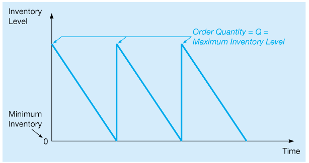
Figure 6.2 Inventory Usage over Time
The annual ordering cost is simply the number of orders per year times the cost of placing each order. Since the inventory level changes daily, it is appropriate to use the average inventory level to determine annual holding or carrying cost. The annual carrying cost will equal the average inventory times the inventory carrying cost per unit per year. Again looking at Figure 6.2, we see that the maximum inventory is the order quantity (Q), and the average inventory will be one-half of that. Table 6.2 provides a numerical example to illustrate this. Notice that for this situation, if the order quantity is 10, the average inventory will be 5, or one-half of Q. Thus:
Table 6.2 Computing Average Inventory
| INVENTORY LEVEL | ||||
|---|---|---|---|---|
| DAY | BEGINNING | ENDING | AVERAGE | |
| April 1 (order received) | 10 | 8 | 9 | |
| April 2 | 8 | 6 | 7 | |
| April 3 | 6 | 4 | 5 | |
| April 4 | 4 | 2 | 3 | |
| April 5 | 2 | 0 | 1 | |
| Maximum level April 1 = 10 units | ||||
| Total of daily averages = 9 + 7 + 5 + 3 + 1 = 25 | ||||
| Number of days = 5 | ||||
| Average inventory level = 25/5 = 5 units | ||||
Using the following variables, we can develop mathematical expressions for the annual ordering and carrying costs:
A graph of the holding cost, the ordering cost, and the total of these two is shown in Figure 6.3. The lowest point on the total cost curves occurs where the ordering cost is equal to the carrying cost. Thus, to minimize total costs, given this situation, the order quantity should occur where these two costs are equal.
Finding the EOQ
When the EOQ assumptions are met, total cost is minimized when:
Solving this for Q gives the optimal order quantity:

Figure 6.3 Total Cost as a Function of Order Quantity
This optimal order quantity is often denoted by Thus, the economic order quantity is given by the following formula:
This EOQ formula is the basis for many more advanced models, and some of these are discussed later in this chapter.
Economic Order Quantity (EOQ) Model
Sumco Pump Company Example
Sumco, a company that sells pump housings to other manufacturers, would like to reduce its inventory cost by determining the optimal number of pump housings to obtain per order. The annual demand is 1,000 units, the ordering cost is $10 per order, and the average carrying cost per unit per year is $0.50. Using these figures, if the EOQ assumptions are met, we can calculate the optimal number of units per order:
The relevant total annual inventory cost is the sum of the ordering cost and the carrying cost:
In terms of the variables in the model, the total cost (TC) can now be expressed as
The total annual inventory cost for Sumco is computed as follows:
The number of orders per year is 5, and the average inventory is 100.
As you might expect, the ordering cost is equal to the carrying cost. You may wish to try different values for Q, such as 100 or 300 pumps. You will find that the minimum total cost occurs when Q is 200 units. The EOQ, is 200 pumps.
Using Excel QM for Basic EOQ Inventory Problems
The Sumco Pump Company example, and a variety of other inventory problems we address in this chapter, can be easily solved using Excel QM. Program 6.1A shows the input data for Sumco and the Excel formulas needed for the EOQ model. Program 6.1B contains the solution for this example, including the optimal order quantity, maximum inventory level, average inventory level, and the number of orders.

Program 6.1A Input Data and Excel QM Formulas for the Sumco Pump Company Example

Program 6.1B Excel QM Solution for the Sumco Pump Company Example
Purchase Cost of Inventory Items
Sometimes the total inventory cost expression is written to include the actual cost of the material purchased. With the EOQ assumptions, the purchase cost does not depend on the particular order policy found to be optimal because, regardless of how many orders are placed each year, we still incur the same annual purchase cost of where C is the purchase cost per unit and D is the annual demand in units.1
It is useful to know how to calculate the average inventory level in dollar terms when the price per unit is given. This can be done as follows. Using the variable Q to represent the quantity of units ordered and assuming a unit cost of C, we can determine the average dollar value of inventory:
This formula is analogous to Equation 6-1.
Many businesses and industries often express the inventory carrying cost as an annual percentage of the unit cost or price. When this is the case, a new variable is introduced. Let I be the annual inventory holding charge as a percent of unit price or cost. Then the cost of storing one unit of inventory for the year, is given by where C is the unit price or cost of an inventory item. can be expressed, in this case, as
Sensitivity Analysis with the EOQ Model
The EOQ model assumes that all input values are fixed and known with certainty. However, since these values are often estimated or may change over time, it is important to understand how the order quantity might change if different input values are used. Determining the effects of these changes is called sensitivity analysis.
The EOQ formula is given as follows:
Because of the square root in the formula, any changes in the inputs will result in relatively minor changes in the optimal order quantity. For example, if were to increase by a factor of 4, the EOQ would increase by only a factor of 2. Consider the Sumco example just presented. The EOQ for this company is as follows:
If we increased from $10 to $40,
In general, the EOQ changes by the square root of a change in any of the inputs.