
11.1 PERT/CPM
Almost any large project can be subdivided into a series of smaller activities or tasks that can be analyzed with PERT/CPM. When you recognize that projects can have thousands of specific activities, you see why it is important to be able to answer questions such as the following:
When will the entire project be completed?
What are the critical activities or tasks in the project—that is, the ones that will delay the entire project if they are late?
Which are the noncritical activities—that is, the ones that can run late without delaying the entire project’s completion?
If there are three time estimates, what is the probability that the project will be completed by a specific date?
At any particular date, is the project on schedule, behind schedule, or ahead of schedule?
On any given date, is the money spent equal to, less than, or greater than the budgeted amount?
Are there enough resources available to finish the project on time?
General Foundry Example of PERT/CPM
General Foundry, Inc., a metalworks plant in Milwaukee, has long been trying to avoid the expense of installing air pollution control equipment. The local environmental protection group has recently given the foundry 16 weeks to install a complex air filter system on its main smokestack. General Foundry was warned that it will be forced to close unless the device is installed in the allotted period. Lester Harky, the managing partner, wants to make sure that installation of the filtering system progresses smoothly and on time.
When the project begins, the building of the internal components for the device (activity A) and the modifications that are necessary for the floor and roof (activity B) can be started. The construction of the collection stack (activity C) can begin once the internal components are completed, and the pouring of the new concrete floor and installation of the frame (activity D) can be completed as soon as the roof and floor have been modified. After the collection stack has been constructed, the high-temperature burner can be built (activity E), and the installation of the pollution control system (activity F) can begin. The air pollution device can be installed (activity G) after the high-temperature burner has been built, the concrete floor has been poured, and the frame has been installed. Finally, after the control system and pollution device have been installed, the system can be inspected and tested (activity H).
All of these activities seem rather confusing and complex until they are placed in a network. First, all of the activities must be listed. This information is shown in Table 11.1. We see in the table that before the collection stack can be constructed (activity C), the internal components must be built (activity A). Thus, activity A is the immediate predecessor of activity C. Similarly, both activities D and E must be performed just prior to installation of the air pollution device (activity G).
Table 11.1 Activities and Immediate Predecessors for General Foundry, Inc.
| ACTIVITY | DESCRIPTION | IMMEDIATE PREDECESSORS |
|---|---|---|
| A | Build internal components | — |
| B | Modify roof and floor | — |
| C | Construct collection stack | A |
| D | Pour concrete and install frame | B |
| E | Build high-temperature burner | C |
| F | Install pollution control system | C |
| G | Install air pollution device | D, E |
| H | Inspect and test pollution control system | F, G |
Drawing the PERT/CPM Network
Once the activities have all been specified (step 1 of the PERT procedure) and management has decided which activities must precede others (step 2), the network can be drawn (step 3).
There are two common techniques for drawing PERT networks. The first is called activity-on-node (AON) because the nodes represent the activities. The second is called activity-on-arc (AOA) because the arcs are used to represent the activities. In this book, we present the AON technique, as this is easier and is often used in commercial software.
In constructing an AON network, there should be one node representing the start of the project and one node representing the finish of the project. There will be one node (represented as a rectangle in this chapter) for each activity. Figure 11.1 gives the entire network for General Foundry. The arcs (arrows) are used to show the predecessors for the activities. For example, the arrows leading into activity G indicate that both D and E are immediate predecessors for G.

Figure 11.1 Network for General Foundry, Inc.
Activity Times
The next step in both CPM and PERT is to assign estimates of the time required to complete each activity. For some projects, such as construction projects, the time to complete each activity may be known with certainty. The developers of CPM assigned just one time estimate to each activity. These times are then used to find the critical path, as described in the sections that follow.
However, for one-of-a-kind projects or for new jobs, providing activity time estimates is not always an easy task. Without solid historical data, managers are often uncertain about the activity times. For this reason, the developers of PERT employed a probability distribution based on three time estimates for each activity. A weighted average of these times is used with PERT in place of the single time estimate used with CPM, and these averages are used to find the critical path. The time estimates in PERT are
Optimistic time (a) time an activity will take if everything goes as well as possible. There should be only a small probability (say, ) of this occurring.
Pessimistic time (b) time an activity will take assuming very unfavorable conditions. There should also be only a small probability that the activity will really take this long.
Most likely time (m) most realistic time estimate to complete the activity.
PERT often assumes that time estimates follow the beta probability distribution (see Figure 11.2). This continuous distribution has been found to be appropriate, in many cases, for determining an expected value and variance for activity completion times.

Figure 11.2 Beta Probability Distribution with Three Time Estimates
To find the expected activity time (t), the beta distribution weights the estimates as follows:
To compute the dispersion or variance of activity completion time, we use this formula:1
Table 11.2 shows General Foundry’s optimistic, most likely, and pessimistic time estimates for each activity. It also reveals the expected time (t) and variance for each of the activities, as computed with Equations 11-1 and 11-2.
Table 11.2 Time Estimates (Weeks) for General Foundry, Inc.
| ACTIVITY | OPTIMISTIC, a | MOST LIKELY, m | PESSIMISTIC, b | EXPECTED TIME, | VARIANCE, |
|---|---|---|---|---|---|
| A | 1 | 2 | 3 | 2 | |
| B | 2 | 3 | 4 | 3 | |
| C | 1 | 2 | 3 | 2 | |
| D | 2 | 4 | 6 | 4 | |
| E | 1 | 4 | 7 | 4 | |
| F | 1 | 2 | 9 | 3 | |
| G | 3 | 4 | 11 | 5 | |
| H | 1 | 2 | 3 | 2 | |
| 25 |
How to Find the Critical Path
Once the expected completion time for each activity has been determined, we accept it as the actual time of that task. Variability in times will be considered later.
Although Table 11.2 indicates that the total expected time for all eight of General Foundry’s activities is 25 weeks, it is obvious in Figure 11.3 that several of the tasks can be taking place simultaneously. To find out just how long the project will take, we perform the critical path analysis for the network.
The critical path is the longest time path route through the network. If Lester Harky wants to reduce the total project time for General Foundry, he will have to reduce the length of some activity on the critical path. Conversely, any delay of an activity on the critical path will delay completion of the entire project.
To find the critical path, we need to determine the following quantities for each activity in the network:
Earliest start time (ES): the earliest time an activity can begin without violation of immediate predecessor requirements
Earliest finish time (EF): the earliest time at which an activity can end
Latest start time (LS): the latest time an activity can begin without delaying the entire project
Latest finish time (LF): the latest time an activity can end without delaying the entire project
In the network, we represent these times, as well as the activity times (t), in the nodes, as seen here:
| ACTIVITY | t |
|---|---|
| ES | EF |
| LS | LF |
We first show how to determine the earliest times. When we find these, the latest times can be computed.
Earliest Times
There are two basic rules to follow when computing ES and EF. The first rule is for the earliest finish time, which is computed as follows:
Also, before any activity can be started, all of its predecessor activities must be completed. In other words, we search for the largest EF for all of the immediate predecessors in determining ES. The second rule is for the earliest start time, which is computed as follows:
The start of the whole project will be set at time zero. Therefore, any activity that has no predecessors will have an earliest start time of zero.So ES = 0 for both A and B in the General Foundry problem, as seen here:


Figure 11.3 General Foundry’s Network with Expected Activity Times
The rest of the earliest times for General Foundry are shown in Figure 11.4. These are found using a forward pass through the network. At each step, and ES is the largest EF of the predecessors. Notice that activity G has an earliest start time of 8, since both D (with ) and E (with ) are immediate predecessors. Activity G cannot start until both predecessors are finished, so we choose the larger of their earliest finish times. Thus, G has The finish time for the project will be 15 weeks, which is the EF for activity H.
Latest Times
The next step in finding the critical path is to compute LS and LF for each activity. We do this by making a backward pass through the network—that is, starting at the finish and working backward.
There are two basic rules to follow when computing the latest times. The first rule involves the latest start time, which is computed as

Figure 11.4 General Foundry’s Earliest Start (ES) and Earliest Finish (EF) Times

Figure 11.5 General Foundry’s Latest Start (LS) and Latest Finish (LF) Times
Also, since all immediate predecessors must be finished before an activity can begin, the latest start time for an activity determines the latest finish time for its immediate predecessors. If an activity is the immediate predecessor for two or more activities, it must be finished so that all following activities can begin by their latest start times. Thus, the second rule involves the latest finish time, which is computed as
To compute the latest times, we start at the finish and work backwards. Since the finish time for the General Foundry project is 15, activity H has The latest start for activity H is
Continuing to work backward, this latest start time of 13 becomes the latest finish time for immediate predecessors F and G. All of the latest times are shown in Figure 11.5. Notice that for activity C, which is the immediate predecessor for two activities (E and F), the latest finish time is the smaller of the latest start times (4 and 10) for activities E and F.
Concept Of Slack In Critical Path Computations
When ES, LS, EF, and LF have been determined, it is a simple matter to find the amount of slack time, or free time, that each activity has. Slack is the length of time an activity can be delayed without delaying the whole project. Mathematically,
Table 11.3 summarizes the ES, EF, LS, LF, and slack time for all of General Foundry’s activities. Activity B, for example, has 1 week of slack time, since (or, similarly, ). This means that it can be delayed up to 1 week without causing the project to run any longer than expected.
On the other hand, activities A, C, E, G, and H have no slack time; this means that none of them can be delayed without delaying the entire project. Because of this, they are called critical activities and are said to be on the critical path. Lester Harky’s critical path is shown in network form in Figure 11.6. The total project completion time (T), 15 weeks, is seen as the largest number in the EF or LF column of Table 11.3. Industrial managers call this a boundary timetable.
Probability of Project Completion
The critical path analysis helped us determine that the foundry’s expected project completion time is 15 weeks. Harky knows, however, that if the project is not completed in 16 weeks, General Foundry will be forced to close by environmental controllers. He is also aware that there is significant variation in the time estimates for several activities. Variation in activities that are on the critical path can affect overall project completion—possibly delaying it. This is one occurrence that worries Harky considerably.
Table 11.3 General Foundry’s Schedule and Slack Times
| ACTIVITY | EARLIEST START, ES | EARLIEST FINISH, EF | LATEST START, LS | LATEST FINISH, LF | SLACK, LS – ES | ON CRITICAL PATH? |
|---|---|---|---|---|---|---|
| A | 0 | 2 | 0 | 2 | 0 | Yes |
| B | 0 | 3 | 1 | 4 | 1 | No |
| C | 2 | 4 | 2 | 4 | 0 | Yes |
| D | 3 | 7 | 4 | 8 | 1 | No |
| E | 4 | 8 | 4 | 8 | 0 | Yes |
| F | 4 | 7 | 10 | 13 | 6 | No |
| G | 8 | 13 | 8 | 13 | 0 | Yes |
| H | 13 | 15 | 13 | 15 | 0 | Yes |
PERT uses the variance of critical path activities to help determine the variance of the overall project. If the activity times are statistically independent, the project variance is computed by summing the variances of the critical activities:
From Table 11.2, we know that
| CRITICAL ACTIVITY | VARIANCE |
|---|---|
| A | |
| C | |
| E | |
| G | |
| H |
Hence, the project variance is

Figure 11.6 General Foundry’s Critical Path (A–C–E–G–H)
We know that the standard deviation is just the square root of the variance, so
How can this information be used to help answer questions regarding the probability of finishing the project on time? In addition to assuming that the activity times are independent, we assume that the total project completion time follows a normal probability distribution. With these assumptions, the bell-shaped curve shown in Figure 11.7 can be used to represent project completion dates. It also means that there is a 50% chance that the entire project will be completed in less than the expected 15 weeks and a 50% chance that it will exceed 15 weeks.2
For Harky to find the probability that his project will be finished on or before the 16-week deadline, he needs to determine the appropriate area under the normal curve. The standard normal equation can be applied as follows:
where
Z = the number of standard deviations the due date or target date lies from the mean or expected completion date

Figure 11.7 Probability Distribution for Project Completion Times
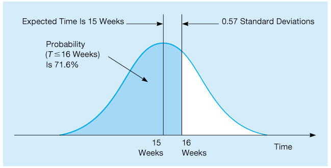
Figure 11.8 Probability of General Foundry’s Meeting the 16-Week Deadline
Referring to the normal table in Appendix A, we find a probability of 0.71566. Thus, there is a 71.6% chance that the pollution control equipment can be put in place in 16 weeks or less. This is shown in Figure 11.8.
What PERT Was Able to Provide
PERT has thus far been able to provide Lester Harky with several valuable pieces of management information:
The project’s expected completion date is 15 weeks.
There is a 71.6% chance that the equipment will be in place within the 16-week deadline. PERT can easily find the probability of finishing by any date Harky is interested in.
Five activities (A, C, E, G, H) are on the critical path. If any one of them is delayed for any reason, the entire project will be delayed.
Three activities (B, D, F) are not critical but have some slack time built in. This means that Harky can borrow from their resources, if needed, possibly to speed up the entire project.
A detailed schedule of activity starting and ending dates has been made available (see Table 11.3).
Using Excel QM for the General Foundry Example
This example can be worked using Excel QM. To do this, select Excel QM from the Add-Ins tab in Excel 2016, as shown in Program 11.1A. In the drop-down menu, put the cursor over Project Management, and choices will appear to the right. To input a problem that is presented in a table with the immediate predecessors and three time estimates, select Predecessor List (AON), and the Initialization window will appear. Specify the number of activities and the maximum number of immediate predecessors for the activities, and select the 3 time estimate option. If you wish to see a Gantt chart, check Graph. Click OK when finished, and a spreadsheet will appear, with all the necessary rows and columns labeled. For this example, enter the three time estimates in cells B8:D15, and then enter the immediate predecessors in cells C18:D25, as shown in Program 11.1B. No other inputs or steps are required.

Program 11.1A Excel QM Initialization Screen for General Foundry Example with Three Time Estimates.
As these data are being entered, Excel QM calculates the expected times and variances for all activities, and a table will automatically display the earliest, latest, and slack times for all the activities. A Gantt chart is displayed, and this chart shows the critical path and slack time for the activities.
Sensitivity Analysis and Project Management
During any project, the time required to complete an activity can vary from the projected or expected time. If the activity is on the critical path, the total project completion time will change, as discussed previously. In addition to having an impact on the total project completion time, there is an impact on the earliest start, earliest finish, latest start, latest finish, and slack times for other activities. The exact impact depends on the relationship among the various activities.
In previous sections, we define an immediate predecessor activity as an activity that comes immediately before a given activity. In general, a predecessor activity is one that must be completed before the given activity can be started. Consider activity G (install air pollution device) for the General Foundry example. As seen previously, this activity is on the critical path. Predecessor activities are A, B, C, D, and E. All of these activities must be completed before activity G can be started. A successor activity is an activity that can be started only after the given activity is finished. Activity H is the only successor activity for activity G. A parallel activity is an activity that does not directly depend on the given activity. Again consider activity G. Are there any parallel activities for this activity? Looking at the network for General Foundry, it can be seen that activity F is a parallel activity of activity G.
After predecessor, successor, and parallel activities have been defined, we can explore the impact that an increase (decrease) in the activity time for a critical path activity would have on other activities in the network. The results are summarized in Table 11.4. If the time it takes to complete activity G increases, there will be an increase in the earliest start, earliest finish, latest start, and latest finish times for all successor activities. Because slack time is equal to the latest finish time minus the earliest finish time (or the latest start time minus the earliest start time; or ), there will be no change in the slack for successor activities. Because activity G is on the critical path, an increase in activity time will increase the total project competition time. This would mean that the latest finish, latest start, and slack times will also increase for all parallel activities. You can prove this to yourself by completing a backward pass through the network using a higher total project completion time. There are no changes for predecessor activities.
