Animating with Dynamics: The Pool Table

This exercise will take you through the creation of a scene in which you’ll use dynamics to animate a cue ball striking two balls on a pool table.

Creating the Pool Table and the Balls

You’ll create a simple pool table as a collision surface for the pool balls. To create the table, follow these steps:

1. Create a polygonal plane for the surface of the table. Scale it to 10 along its height and length.

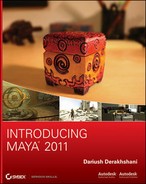
2. To create the pocket holes, make two holes in opposite corners. The easiest way is to duplicate the tabletop plane and offset it slightly in both directions, as shown in Figure 12-3. Doing so creates a pair of square holes in the corners for the ball to drop through. For this exercise, it will do perfectly well.

3. Create a polygonal cube, and scale it to fit one edge of the plane to create a rail. Duplicate the cube three times, and then move and rotate the pieces to create the rails around the table, as shown in Figure 12-4.

Figure 12-3: Duplicate the tabletop plane, and offset it slightly in both directions.

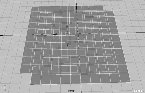
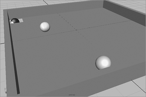
Figure 12-4: A simple pool table

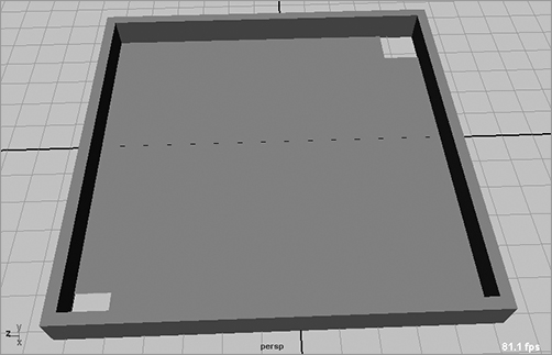
4. Create three poly spheres, and then scale and place them as shown in Figure 12-5. It’s important to place them slightly above the pool table surface. Although it’s not imperative to have the exact location shown in the figure, it’s a good idea to get close to the layout shown.

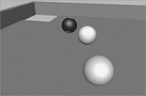
5. Shade your pool balls to make each one different. The figures in this exercise show a solid white ball, a striped ball (it will be yellow on your screen), and a black eight ball, as shown in Figure 12-6.

Figure 12-5: Scaling and placing the three spheres

Figure 12-6: The pool balls in texture view

The spheres are placed a bit over the table surface so that their geometries’ surfaces aren’t accidentally crossing each other, an effect known as interpenetrating. When surfaces interpenetrate, the dynamics that result are usually as welcome as sand in your eyes. Starting all colliding rigid bodies slightly away from each other should guarantee that their surfaces don’t interpenetrate. Using the simple pool table that you’ve set up will make the dynamics calculations quick and easy.

Use the file Table_v1.mb in the Scenes folder of the Pool_Table project on the CD as a reference or to catch up to this point.

Creating Rigid Bodies

Define the pool table as a passive rigid body, and define the pool balls as active rigid bodies. Follow these steps:

Animating Rigid Bodies

If you need to, enable texture view in your view panel by pressing 6.

The next step is to put the cue ball (the white sphere) into motion so that it hits the striped ball into the black eight ball to sink it into the corner pocket. The easiest way to do this is to keyframe the cue ball’s translation from its starting point to hit into the striped ball. However, because active rigid bodies can’t be keyframed, you have to turn the cue ball into a passive rigid body. To do that, follow these steps:

Figure 12-7: Move the cue ball with the Translate tool.

By animating the ball as a passive rigid body, keyframing its translation, and then turning it back to active, you set the dynamic simulation in motion. The cue ball animates from its starting position and hits the striped ball. Maya’s dynamics engine calculates the collisions on that ball and sets it into motion; the ball then strikes the black eight ball, which should roll into the corner pocket. The dynamics engine, at frame 11, also calculates the movement of the cue ball after it strikes the striped ball, so you don’t have to animate its ricochet.

Go to the start frame, and play back the simulation. The cue ball knocks the striped ball into the eight ball. The eight ball rolls into the corner, and the striped ball bounces off to the right. If the eight ball doesn’t go into the corner, you’ll have to edit your cue ball’s keyframes to hit the striped ball at the correct angle to hit the eight ball into the corner pocket.

At the current settings, however, the eight ball bounces out of the corner without falling through the hole. You need to control the bounciness of the collisions:

Figure 12-8: The eight ball falls through the hole.

You can load the scene file Table_v2.mb from the Pool_Table project on the CD to compare your work.

Additional Rigid Body Attributes

In addition, while using the pool table setup without any animation, try playing with the rigid body attributes to see how they affect the rigid body in question. Some of these attributes are defined here:

Initial Velocity Gives the rigid body an initial push to move it in the corresponding axis.

Initial Spin Gives the rigid body object an initial twist to start the rotation of the object in that axis.

Impulse Position Gives the object a constant push in that axis. The effect is cumulative; the object will accelerate if the impulse isn’t turned off.

Spin Impulse Rotates the object constantly in the desired axis. The spin will accelerate if the impulse isn’t turned off.

Center of Mass (0,0,0) Places the center of the object’s mass at its pivot point, typically at its geometric center. This value offsets the center of mass, so the rigid body object behaves as if its center of balance is offset, like trick dice or a top-weighted ball.

Creating animation with rigid bodies is straightforward and can go a long way toward creating natural-looking motion for your scene. Integrating such animation into a final project can become fairly complicated, though, so it’s prudent to become familiar with the workings of rigid body dynamics before relying on that sort of workflow for an animated project. You’ll find that most professionals use rigid body dynamics as a springboard to create realistic motion for their projects. The dynamics are often converted to keyframes and further tweaked by the animator to fit into a larger scene.

Here are a few suggestions for scenes using rigid body dynamics:

Bowling Lane The bowling ball is keyframed as a passive object until it hits the active rigid pins at the end of the lane. This scene is simple to create and manipulate.

Dice Active rigid dice are thrown into a passive rigid craps table. This exercise challenges your dynamics abilities as well as your modeling skills if you create an accurate craps table.

Game of Marbles This scene challenges your texturing and rendering abilities as well as your dynamics abilities.

Baking Out a Simulation

Frequently, a dynamic simulation is created to fit into another scene, perhaps to interact with other objects and such. In instances such as this, you want to exchange the dynamic properties of the dynamic body you have set up in a simulation for regular, good old-fashioned animation curves that you can edit along with the rest of the animated scene, if need be. You can easily take a simulation that you’ve created and bake it out to curves. As much fun as it is to think of cupcakes, baking is a somewhat catchall term used to describe converting one type of action or procedure into another; in this case, you’re baking dynamics into keyframes.

You’ll take the simulation you set up with the pool balls earlier and turn them into keyframes to give you a quick idea of how it can be done and the curves that you’ll get. Dynamics is a deep layer of Maya, and there is a lot to learn about it. Keep in mind that you can use this introduction as a foundation for your own explorations.

To bake out the rigid body simulation of the pool balls, follow these steps:

1. Open the scene file Table_v2.mb from the Pool_Table project on the CD; or, if you prefer, open your scene from the previous exercise. You’ll bake out the motion of all three pool balls on the table to see their keyframes.

2. Because the simulation is already set up and working to your liking, you can jump right to it. Select all three pool balls, and choose Edit ⇒ Keys ⇒ Bake Simulation ❒. In the option box, as shown in Figure 12-9, set Time Range to Time Slider (which should be set to 1 to 150). This, of course, sets the range you would like to bake into curves.

3. Set Hierarchy to Selected, and set Channels to From Channel Box. This ensures that you have control over which keys are created. Make sure Keep Unbaked Keys and Disable Implicit Control are checked and that Sparse Curve Bake is turned off. Before clicking the Bake or Apply button, select the Translate and Rotate channels in the Channel Box. Click Bake.

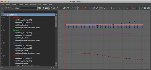
4. Maya runs through the simulation. Scrub the timeline back and forth. Notice how the pool balls move around normally as if the dynamic simulation were running—except that you can scrub in the timeline, which you can’t do with a dynamics simulation. If you open the Graph Editor, you’ll see something similar to Figure 12-10.

Figure 12-9: The Bake Simulation Options window

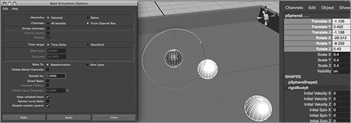
Figure 12-10: The pool balls have animation curves.

5. The curves are crowded; they have keyframes at every frame. A typical dynamics bake gives results like this. But you can set the Bake command to sparse the curves for you; that is, it can take out keyframes at frames that have values within a certain tolerance, so that a minor change in the ball’s position or rotation need not have a keyframe on the curve.

6. Let’s go back in time and try this again. Press Z (Undo) until you back up to right before you baked out the simulation to curves. You can also close this scene and reopen it from the original project, if necessary. This time, select the balls, and choose Edit ⇒ Keys ⇒ Bake Simulation ❒. In the option box, turn on the Sparse Curve Bake setting, and set Sample By to 5. Select the channels in the Channel Box, and click Bake. You’re telling Maya to only look at every five frames of the simulation to set keyframes.

7. Maya runs through the simulation again and bakes everything out to curves. This time it makes a sparser animation curve for each channel because it’s looking at five-frame intervals, as shown in Figure 12-11. If you open the Graph Editor, you’ll notice that the curves are much friendlier to look at and edit.

Figure 12-11: Sampling by fives makes a cleaner curve.

Sampling by fives may give you an easier curve to edit, but it can overly simplify the animation of your objects; make sure you use the best Sampling setting for your simulation when you need to convert it to curves for editing.

Simplifying Animation Curves

Despite a higher Sampling setting when you bake out the simulation, you can still be left with a lot of keyframes to deal with, especially if you have to modify the animation extensively from here. One last trick you can use is to simplify the curve further through the Graph Editor. You have to work with curves of the same relative size, so you’ll start with the rotation curves, because they have larger values. To keep things simple, let’s deal with one ball: the black eight ball. To simplify the curve in the Graph Editor, follow these steps:

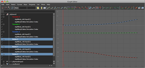
1. Select the black eight ball, and open the Graph Editor. In the left Outliner side, select Rotate.X, Rotate.Y, and Rotate.Z to display only these curves in the graph view. Figure 12-12 shows the curves.

Figure 12-12: The Graph Editor displays the rotation curves of the eight ball.

2. In the left panel of the Graph Editor, select the rigidBody_rx8.Input(1) nodes displayed under the Rotate X, Y, and Z entries for all three curves, as shown in Figure 12-13. In the Graph Editor menu, choose Curves ⇒ Simplify Curve ❒. In the option box, set Time Range to All, set Simplify Method to Dense Data, set Time Tolerance to 0.2, and set Value Tolerance to 0.5. These are fairly high values, but because you’re dealing with rotation of the ball, the degree values are high enough. For more intricate values such as translation, you would use much lower tolerances when simplifying a curve.

3. Click Simplify, and you see that the curve retains its basic shape but loses some of the unneeded keyframes. Figure 12-14 shows the simplified curve, which differs little from the original curve with keys at every five frames.

Figure 12-13: Select the curves to simplify them.

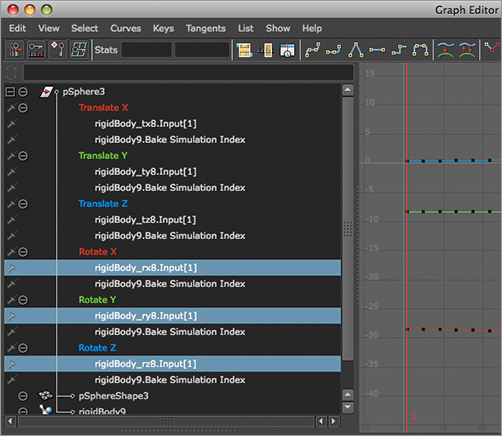
Figure 12-14: A simplified curve for the rotations of the eight ball

Simplifying curves is a handy way to convert a dynamic simulation to curves. But you can also use this method to simplify other animation curves, to make it easier to edit them as you animate the scene. Keep in mind that you may lose fidelity to the original animation after you simplify a curve, so use this technique with care.

With this methodology, you can bake out the animation of any simulation, from dynamics (as you just did) to constraints and some scripts. The curve simplification works with good old-fashioned keyframed curves as well; if you inherit a scene from another animator and need to simplify the curves, do it just as you did here.